Surface visualization 

Table of Contents

Surface visualization

This section describes the whereabouts of the main surfaces generated by the pipeline, and how you can visualized them using python or R. This example will use the subject HC001 and session 01 from the MICs dataset, and all paths will be relative to the subject directory or out/micapipe/sub-HC001_ses01/

In the following examples, we’ll load and visualize single subject surfaces. Surfaces are distributed across different directories, namely:

sub-HC001/
└── ses-01
    ├── surf   # fsnative, fsaverage5, fsLR-32k, fsLR-5k surfaces**
    └── maps   # Thickness, curvature and quantitative maps**

Each native surface parcellation is found inside the subject’s freesurfer directory and contains the string mics.annot:

freesurfer/
└── sub-HC001_ses-01
    └── label
        ├── lh.schaefer-400_**mics.annot**
        └── rh.schaefer-400_**mics.annot**

Setting the environment 

This example uses the packages the python packages os, matplotlib, numpy, nibabel, matplotlib and brainspace. If you are interested in plotting surfaces with BrainSpace, check the corresponding documentation!!

R libraries are RColorBrewer, viridis, fsbrain, freesurferformats and rgl. For further information about managing and visualizing surfaces with R, check the fsbrain vignettes, fsbrain github repository, and freesurferformats

The first step in both languages is to set the environment.

# Set the environment
import os
import glob
import numpy as np
import nibabel as nib
import seaborn as sns
from brainspace.plotting import plot_hemispheres
from brainspace.mesh.mesh_io import read_surface
from brainspace.datasets import load_conte69

# Set the working directory to the 'out' directory
out='/data_/mica3/BIDS_MICs/derivatives' # <<<<<<<<<<<< CHANGE THIS PATH
os.chdir(out)

# This variable will be different for each subject
sub='sub-HC001'
ses='ses-01'
subjectID=f'{sub}_{ses}'           # <<<<<<<<<<<< CHANGE THIS SUBJECT's ID
subjectDir=f'micapipe_v0.2.0/{sub}/{ses}' # <<<<<<<<<<<< CHANGE THIS SUBJECT's DIRECTORY

# Set paths and variables
dir_FS = 'freesurfer/' + subjectID
dir_surf = subjectDir + '/surf/'
dir_maps = subjectDir + '/maps/'

# Path to MICAPIPE
micapipe=os.popen("echo $MICAPIPE").read()[:-1]

# Set the environment        'R 4.3.1'
require('RColorBrewer')      # version 1.1.3
require('viridis')           # version 0.6.5
require('fsbrain')           # version 0.5.5
require('freesurferformats') # version 0.1.18
require('rgl')               # version 1.2.8
require('gifti')             # version 0.8.0

# Define working directory and subject-specific information. CHANGE THESE      PATHS as appropriate.
setwd('~/derivatives_RtD/')                      # working directory
subjectID <- 'sub-HC001_ses-01'                  # subject ID
subjectDir <- 'micapipe_v0.2.0/sub-HC001/ses-01' # subject directory path

# Set paths for surface and morphometry data.
dir_surf <- paste0(subjectDir, '/surf/')
dir_maps <- paste0(subjectDir, '/maps/')

Load the surfaces 

# Load native pial surface
pial_lh = read_surface(dir_FS+'/surf/lh.pial', itype='fs')
pial_rh = read_surface(dir_FS+'/surf/rh.pial', itype='fs')

# Load native white matter surface
wm_lh = read_surface(dir_FS+'/surf/lh.white', itype='fs')
wm_rh = read_surface(dir_FS+'/surf/rh.white', itype='fs')

# Load native inflated surface
inf_lh = read_surface(dir_FS+'/surf/lh.inflated', itype='fs')
inf_rh = read_surface(dir_FS+'/surf/rh.inflated', itype='fs')

# Load fsaverage5
fs5_lh = read_surface('freesurfer/fsaverage5/surf/lh.pial', itype='fs')
fs5_rh = read_surface('freesurfer/fsaverage5/surf/rh.pial', itype='fs')

# Load fsaverage5 inflated
fs5_inf_lh = read_surface('freesurfer/fsaverage5/surf/lh.inflated', itype='fs')
fs5_inf_rh = read_surface('freesurfer/fsaverage5/surf/rh.inflated', itype='fs')

# Load fsLR 32k
f32k_lh = read_surface(micapipe + '/surfaces/fsLR-32k.L.surf.gii', itype='gii')
f32k_rh = read_surface(micapipe + '/surfaces/fsLR-32k.R.surf.gii', itype='gii')

# Load fsLR 32k inflated
f32k_inf_lh = read_surface(micapipe + '/surfaces/fsLR-32k.L.inflated.surf.gii', itype='gii')
f32k_inf_rh = read_surface(micapipe + '/surfaces/fsLR-32k.R.inflated.surf.gii', itype='gii')

# Load Load fsLR 5k
f5k_lh = read_surface(micapipe + '/surfaces/fsLR-5k.L.surf.gii', itype='gii')
f5k_rh = read_surface(micapipe + '/surfaces/fsLR-5k.R.surf.gii', itype='gii')

# Load fsLR 5k inflated
f5k_inf_lh = read_surface(micapipe + '/surfaces/fsLR-5k.L.inflated.surf.gii', itype='gii')
f5k_inf_rh = read_surface(micapipe + '/surfaces/fsLR-5k.R.inflated.surf.gii', itype='gii')

# Helper function to plot brain surfaces
plot_surface <-function(brainMesh, legend='', view_angles=c('sd_lateral_lh', 'sd_medial_lh', 'sd_medial_rh', 'sd_lateral_rh'), img_only=FALSE) {
  try(img <- vis.export.from.coloredmeshes(brainMesh, colorbar_legend = legend, grid_like = FALSE, view_angles = view_angles, img_only = img_only, horizontal=TRUE))
  while (rgl.cur() > 0) { rgl.close() }; file.remove(list.files(path = getwd(), pattern = 'fsbrain'))
  return(img)
}

# Define color maps for brain visualization.
RdYlGn <- colorRampPalette(brewer.pal(11,'RdYlGn'))
bw <- colorRampPalette(c('black','gray65', 'white'))
grays <- colorRampPalette(c('gray65', 'gray65', 'gray65'))

# Set color limits for data visualization
lft = limit_fun(1.5, 4)    # thickness color scale
lfc = limit_fun(-0.2, 0.2) # curvature color scale

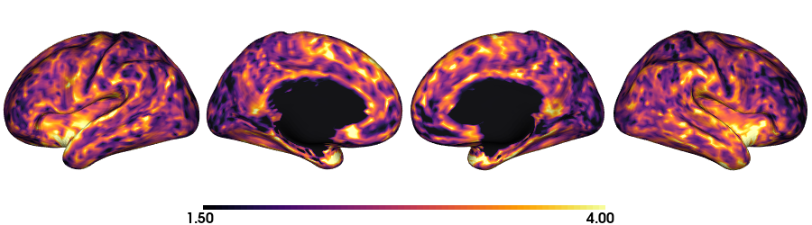
Morphology 

Two surface based morphological features are plotted here: cortical thickness and curvature. Both measurements are generates in three main surfaces, native, fsaverage5, fsLR-32k and fsLR-5k.

Thickness: Inflated native surface 

# Load data
th_lh = dir_maps + subjectID + '_hemi-L_surf-fsnative_label-thickness.func.gii'
th_rh = dir_maps + subjectID + '_hemi-R_surf-fsnative_label-thickness.func.gii'
th_nat = np.hstack(np.concatenate((nib.load(th_lh).darrays[0].data,
                                   nib.load(th_rh).darrays[0].data), axis=0))

# Plot the surface
plot_hemispheres(inf_lh, inf_rh, array_name=th_nat, size=(900, 250), color_bar='bottom', zoom=1.25, embed_nb=True, interactive=False, share='both',
                 nan_color=(0, 0, 0, 1), color_range=(1.5, 4), cmap="inferno", transparent_bg=False)

# Define paths for left and right hemisphere thickness data using FreeSurfer's native format (fsnative).
th.lh <- paste0(dir_maps, subjectID, "_hemi-L_surf-fsnative_label-thickness.func.gii")
th.rh <- paste0(dir_maps, subjectID, "_hemi-R_surf-fsnative_label-thickness.func.gii")

# Use 'vis.data.on.subject' to visualize thickness data on the inflated cortical surface, specific to FreeSurfer format.
th_nat <- vis.data.on.subject('freesurfer', subjectID, morph_data_lh=th.lh, morph_data_rh=th.rh, surface='inflated', draw_colorbar = TRUE,
                              views=NULL, rglactions = list('trans_fun'=limit_fun(1.5, 4), 'no_vis'=T),  makecmap_options = list('colFn'=inferno))

# Display the native surface with mapped thickness data.
plot_surface(th_nat, 'Thickness [mm]')

Thickness: `fsaverage5`

# Load data
th_lh_fs5 = dir_maps + subjectID + '_hemi-L_surf-fsaverage5_label-thickness.func.gii'
th_rh_fs5 = dir_maps + subjectID + '_hemi-R_surf-fsaverage5_label-thickness.func.gii'
th_fs5 = np.hstack(np.concatenate((nib.load(th_lh_fs5).darrays[0].data,
                                   nib.load(th_rh_fs5).darrays[0].data), axis=0))

# Plot the surface
plot_hemispheres(fs5_inf_lh, fs5_inf_rh, array_name=th_fs5, size=(900, 250), color_bar='bottom', zoom=1.25, embed_nb=True, interactive=False, share='both',
                         nan_color=(0, 0, 0, 1), color_range=(1.5, 4), cmap="inferno", transparent_bg=False)

# This section provides a pathway for visualizing thickness without requiring FreeSurfer-formatted surfaces, utilizing the fsaverage5 template.
# Load fsaverage5 surface paths for left and right hemispheres.
fs5.lh <-  read.fs.surface(filepath = 'micapipe/surfaces/fsaverage5/surf/lh.inflated')
fs5.rh <-  read.fs.surface(filepath = 'micapipe/surfaces/fsaverage5/surf/rh.inflated')

# Define paths for thickness morphometric data on fsaverage5 for each hemisphere.
fs5.lh.th <- paste0(dir_maps, subjectID, '_hemi-L_surf-fsaverage5_label-thickness.func.gii')
fs5.rh.th <- paste0(dir_maps, subjectID, '_hemi-R_surf-fsaverage5_label-thickness.func.gii')

# Create colored meshes for both hemispheres based on thickness data.
cml.fs5.th <- coloredmesh.from.preloaded.data(fs5.lh, morph_data = lft(unlist(readgii(fs5.lh.th)$data)), hemi = 'lh', makecmap_options = list('colFn'=inferno))
cmr.fs5.th <- coloredmesh.from.preloaded.data(fs5.rh, morph_data = lft(unlist(readgii(fs5.rh.th)$data)), hemi = 'rh', makecmap_options = list('colFn'=inferno))
th_fs5 <- brainviews(views = 't4', coloredmeshes=list('lh'=cml.fs5.th, 'rh'=cmr.fs5.th), rglactions = list('no_vis'=T))

# Display the fsaverage5 surface with thickness data.
plot_surface(th_fs5, 'Thickness [mm]')

Thickness: `fsLR-32k`

# Load the data
th_lh_fsLR32k = dir_maps + subjectID + '_hemi-L_surf-fsLR-32k_label-thickness.func.gii'
th_rh_fsLR32k = dir_maps + subjectID + '_hemi-R_surf-fsLR-32k_label-thickness.func.gii'
th_fsLR32k = np.hstack(np.concatenate((nib.load(th_lh_fsLR32k).darrays[0].data,
                                       nib.load(th_rh_fsLR32k).darrays[0].data), axis=0))

# Plot the surface
plot_hemispheres(f32k_inf_lh, f32k_inf_rh, array_name=th_fsLR32k, size=(900, 250), color_bar='bottom', zoom=1.25, embed_nb=True, interactive=False, share='both',
                         nan_color=(0, 0, 0, 1), color_range=(1.5, 4), cmap="inferno", transparent_bg=False)

# Load fsLR-32k surface paths for left and right hemispheres.
f32k.lh <-  read.fs.surface(filepath = 'micapipe/surfaces/fsLR-32k.L.surf.gii', format = "gii")
f32k.rh <-  read.fs.surface(filepath = 'micapipe/surfaces/fsLR-32k.R.surf.gii', format = "gii")

# Define paths for thickness morphometry data on fsLR-32k for each hemisphere.
f32k.lh.th <- paste0(dir_maps, subjectID, '_hemi-L_surf-fsLR-32k_label-thickness.func.gii')
f32k.rh.th <- paste0(dir_maps, subjectID, '_hemi-R_surf-fsLR-32k_label-thickness.func.gii')

# Create colored meshes based on thickness data.
cml.f32k.th <- coloredmesh.from.preloaded.data(f32k.lh, morph_data = lft(unlist(readgii(f32k.lh.th)$data)), hemi = 'lh', makecmap_options = list('colFn'=inferno))
cmr.f32k.th <- coloredmesh.from.preloaded.data(f32k.rh, morph_data = lft(unlist(readgii(f32k.rh.th)$data)), hemi = 'rh', makecmap_options = list('colFn'=inferno))
th_f32k <- brainviews(views = 't4', coloredmeshes=list('lh'=cml.f32k.th, 'rh'=cmr.f32k.th), rglactions = list('no_vis'=T))

# Display the fsLR-32k surface with thickness data.
plot_surface(th_f32k, 'Thickness [mm]')

Thickness: `fsLR-5k`

# Load the data
th_lh_fsLR5k = dir_maps + subjectID + '_hemi-L_surf-fsLR-5k_label-thickness.func.gii'
th_rh_fsLR5k = dir_maps + subjectID + '_hemi-R_surf-fsLR-5k_label-thickness.func.gii'
th_fsLR5k = np.hstack(np.concatenate((nib.load(th_lh_fsLR5k).darrays[0].data,
                                       nib.load(th_rh_fsLR5k).darrays[0].data), axis=0))

# Plot the surface
plot_hemispheres(f5k_inf_lh, f5k_inf_rh, array_name=th_fsLR5k, size=(900, 250), color_bar='bottom', zoom=1.25, embed_nb=True, interactive=False, share='both',
                         nan_color=(0, 0, 0, 1), color_range=(1.5, 4), cmap="inferno", transparent_bg=False)

# Load fsLR-5k surface paths for left and right hemispheres.
f5k.lh <-  read.fs.surface(filepath = 'micapipe/surfaces/fsLR-5k.L.surf.gii', format = "gii")
f5k.rh <-  read.fs.surface(filepath = 'micapipe/surfaces/fsLR-5k.R.surf.gii', format = "gii")

# Define paths for thickness morphometry data on fsLR-5k for each hemisphere.
f5k.lh.th <- paste0(dir_maps, subjectID, '_hemi-L_surf-fsLR-5k_label-thickness.func.gii')
f5k.rh.th <- paste0(dir_maps, subjectID, '_hemi-R_surf-fsLR-5k_label-thickness.func.gii')

# Create colored meshes based on thickness data.
cml.f5k.th <- coloredmesh.from.preloaded.data(f5k.lh, morph_data = lft(unlist(readgii(f5k.lh.th)$data)), hemi = 'lh', makecmap_options = list('colFn'=inferno))
cmr.f5k.th <- coloredmesh.from.preloaded.data(f5k.rh, morph_data = lft(unlist(readgii(f5k.rh.th)$data)), hemi = 'rh', makecmap_options = list('colFn'=inferno))
th_f5k <- brainviews(views = 't4', coloredmeshes=list('lh'=cml.f5k.th, 'rh'=cmr.f5k.th), rglactions = list('no_vis'=T))

# Display the fsLR-5k surface with thickness data.
plot_surface(th_f5k, 'Thickness [mm]')

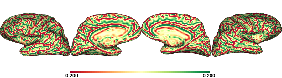
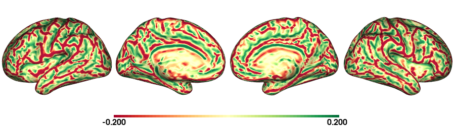
Curvature: Native inflated surface 

# Load the data
cv_lh = dir_maps + subjectID + '_hemi-L_surf-fsnative_label-curv.func.gii'
cv_rh = dir_maps + subjectID + '_hemi-R_surf-fsnative_label-curv.func.gii'
cv = np.hstack(np.concatenate((nib.load(cv_lh).darrays[0].data,
                               nib.load(cv_rh).darrays[0].data), axis=0))

# Plot the surface
plot_hemispheres(inf_lh, inf_rh, array_name=cv, size=(900, 250), color_bar='bottom', zoom=1.25, embed_nb=True, interactive=False, share='both',
                         nan_color=(0, 0, 0, 1), color_range=(-0.2, 0.2), cmap='RdYlGn', transparent_bg=False)

# Define paths for left and right hemisphere curvature data in FreeSurfer's native format (fsnative).
cv.lh <- paste0(dir_maps, subjectID, '_hemi-L_surf-fsnative_label-curv.func.gii')
cv.rh <- paste0(dir_maps, subjectID, '_hemi-R_surf-fsnative_label-curv.func.gii')

# Use 'vis.data.on.subject' to visualize curvature on the subject's inflated surface.
cv_nat <- vis.data.on.subject('freesurfer/', subjectID, morph_data_lh=cv.lh, morph_data_rh=cv.rh, surface='inflated', draw_colorbar = TRUE,
                              views=NULL, rglactions = list('trans_fun'=limit_fun(-0.2, 0.2), 'no_vis'=T),  makecmap_options = list('colFn'=RdYlGn))

# Display the native surface with mapped curvature data.
plot_surface(cv_nat, 'Curvature [1/mm]')

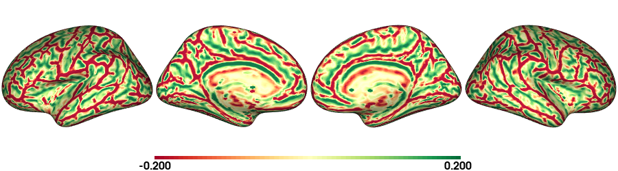
Curvature: `fsaverage5`

# Load the data
cv_lh_fs5 = dir_maps + subjectID + '_hemi-L_surf-fsaverage5_label-curv.func.gii'
cv_rh_fs5 = dir_maps + subjectID + '_hemi-R_surf-fsaverage5_label-curv.func.gii'
cv_fs5 = np.hstack(np.concatenate((nib.load(cv_lh_fs5).darrays[0].data,
                                   nib.load(cv_rh_fs5).darrays[0].data), axis=0))

# Plot the surface
plot_hemispheres(fs5_inf_lh, fs5_inf_rh, array_name=cv_fs5, size=(900, 250), color_bar='bottom', zoom=1.25, embed_nb=True, interactive=False, share='both',
                         nan_color=(0, 0, 0, 1), color_range=(-0.2, 0.2), cmap='RdYlGn', transparent_bg=False)

# Load fsaverage5 surface paths for left and right hemispheres.
fs5.lh <- read.fs.surface(filepath = 'micapipe/surfaces/fsaverage5/surf/lh.inflated')
fs5.rh <- read.fs.surface(filepath = 'micapipe/surfaces/fsaverage5/surf/rh.inflated')

# Define paths to the morphometry data on fsaverage5.
fs5.lh.cv <- paste0(dir_maps, subjectID, '_hemi-L_surf-fsaverage5_label-curv.func.gii')
fs5.rh.cv <- paste0(dir_maps, subjectID, '_hemi-R_surf-fsaverage5_label-curv.func.gii')

# Generate colored meshes using morphometry data.
cml_fs5 <- coloredmesh.from.preloaded.data(fs5.lh, morph_data = lfc(unlist(readgii(fs5.lh.cv)$data)), hemi = 'lh', makecmap_options = list('colFn'=RdYlGn))
cmr_fs5 <- coloredmesh.from.preloaded.data(fs5.rh, morph_data = lfc(unlist(readgii(fs5.rh.cv)$data)), hemi = 'rh', makecmap_options = list('colFn'=RdYlGn))
cv_fs5 <- brainviews(views = 't4', coloredmeshes=list('lh'=cml_fs5, 'rh'=cmr_fs5), rglactions = list('no_vis'=T))

# Display the fsaverage5 surface with morphometry data.
plot_surface(cv_fs5, 'Curvature [1/mm]')

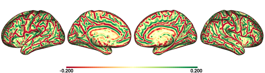
Curvature: `fsLR-32k`

# Load the data
cv_lh_fsLR32k = dir_maps + subjectID + '_hemi-L_surf-fsLR-32k_label-curv.func.gii'
cv_rh_fsLR32k = dir_maps + subjectID + '_hemi-R_surf-fsLR-32k_label-curv.func.gii'
cv_fsLR32k = np.hstack(np.concatenate((nib.load(cv_lh_fsLR32k).darrays[0].data,
                                       nib.load(cv_rh_fsLR32k).darrays[0].data), axis=0))
# Plot the surface
plot_hemispheres(f32k_inf_lh, f32k_inf_rh, array_name=cv_fsLR32k, size=(900, 250), color_bar='bottom', zoom=1.25, embed_nb=True, interactive=False, share='both',
                         nan_color=(0, 0, 0, 1), color_range=(-0.2, 0.2), cmap='RdYlGn', transparent_bg=False)

# Load fsLF-32k surface paths for left and right hemispheres.
f32k.lh <- read.fs.surface(filepath = 'micapipe/surfaces/fsLR-32k.L.inflated.surf.gii')
f32k.rh <- read.fs.surface(filepath = 'micapipe/surfaces/fsLR-32k.R.inflated.surf.gii')

# Define paths to the morphometry data on fsLF32k.
f32k.lh.cv <- paste0(dir_maps, subjectID, '_hemi-L_surf-fsLR-32k_label-curv.func.gii')
f32k.rh.cv <- paste0(dir_maps, subjectID, '_hemi-R_surf-fsLR-32k_label-curv.func.gii')

# Generate colored meshes using morphometry data.
cml_f32k <- coloredmesh.from.preloaded.data(f32k.lh, morph_data = lfc(unlist(readgii(f32k.lh.cv)$data)), hemi = 'lh', makecmap_options = list('colFn'=RdYlGn))
cmr_f32k <- coloredmesh.from.preloaded.data(f32k.rh, morph_data = lfc(unlist(readgii(f32k.rh.cv)$data)), hemi = 'rh', makecmap_options = list('colFn'=RdYlGn))
cv.f32k <- brainviews(views = 't4', coloredmeshes=list('lh'=cml_f32k, 'rh'=cmr_f32k), rglactions = list('no_vis'=T))

# Display the fsLR-32k surface with morphometry data.
plot_surface(cv.f32k, 'Curvature [1/mm]')

Curvature: `fsLR-5k`

# Load the data
cv_lh_fsLR5k = dir_maps + subjectID + '_hemi-L_surf-fsLR-5k_label-curv.func.gii'
cv_rh_fsLR5k = dir_maps + subjectID + '_hemi-R_surf-fsLR-5k_label-curv.func.gii'
cv_fsLR5k = np.hstack(np.concatenate((nib.load(cv_lh_fsLR5k).darrays[0].data,
                                       nib.load(cv_rh_fsLR5k).darrays[0].data), axis=0))
# Plot the surface
plot_hemispheres(f5k_inf_lh, f5k_inf_rh, array_name=cv_fsLR5k, size=(900, 250), color_bar='bottom', zoom=1.25, embed_nb=True, interactive=False, share='both',
                         nan_color=(0, 0, 0, 1), color_range=(-0.2, 0.2), cmap='RdYlGn', transparent_bg=False)

# Load fsLF-5k surface paths for left and right hemispheres.
f5k.lh <- read.fs.surface(filepath = 'micapipe/surfaces/fsLR-5k.L.inflated.surf.gii')
f5k.rh <- read.fs.surface(filepath = 'micapipe/surfaces/fsLR-5k.R.inflated.surf.gii')

# Define paths to the morphometry data on fsLR-5k.
f5k.lh.cv <- paste0(dir_maps, subjectID, '_hemi-L_surf-fsLR-5k_label-curv.func.gii')
f5k.rh.cv <- paste0(dir_maps, subjectID, '_hemi-R_surf-fsLR-5k_label-curv.func.gii')

# Generate colored meshes using morphometry data.
cml_f5k <- coloredmesh.from.preloaded.data(f5k.lh, morph_data = lfc(unlist(readgii(f5k.lh.cv)$data)), hemi = 'lh', makecmap_options = list('colFn'=RdYlGn))
cmr_f5k <- coloredmesh.from.preloaded.data(f5k.rh, morph_data = lfc(unlist(readgii(f5k.rh.cv)$data)), hemi = 'rh', makecmap_options = list('colFn'=RdYlGn))
cv.f5k <- brainviews(views = 't4', coloredmeshes=list('lh'=cml_f5k, 'rh'=cmr_f5k), rglactions = list('no_vis'=T))

# Display the fsLR-5k surface with morphometry data.
plot_surface(cv.f5k, 'Curvature [1/mm]')

`fsLR-32k`

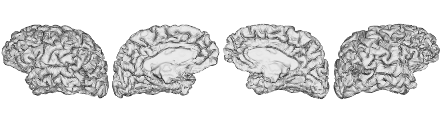
`fsLR-32k`: Pial surface 

# Native conte69 pial surface
fsLR32k_pial_lh = read_surface(dir_surf+subjectID+'_hemi-L_space-nativepro_surf-fsLR-32k_label-pial.surf.gii', itype='gii')
fsLR32k_pial_rh = read_surface(dir_surf+subjectID+'_hemi-R_space-nativepro_surf-fsLR-32k_label-pial.surf.gii', itype='gii')

# Plot the surface
plot_hemispheres(fsLR32k_pial_lh, fsLR32k_pial_rh, size=(900, 250), zoom=1.25, embed_nb=True, interactive=False, share='both',
                 nan_color=(0, 0, 0, 1), color_range=(1.5, 4), cmap='Greys', transparent_bg=False)

# Load fsLR-32k pial surfaces for left and right hemispheres.
f32k.pial.lh <- read.fs.surface(filepath = paste0(dir_surf, subjectID,'_hemi-L_space-nativepro_surf-fsLR-32k_label-pial.surf.gii') )
f32k.pial.rh <- read.fs.surface(filepath = paste0(dir_surf, subjectID,'_hemi-R_space-nativepro_surf-fsLR-32k_label-pial.surf.gii') )

# Prepare and plot the surfaces for visualization.
cml = coloredmesh.from.preloaded.data(f32k.pial.lh, morph_data = rnorm(nrow(f32k.pial.lh$vertices),5,1), makecmap_options = list('colFn'=grays) )
cmr = coloredmesh.from.preloaded.data(f32k.pial.rh, morph_data = rnorm(nrow(f32k.pial.rh$vertices),5,1), makecmap_options = list('colFn'=grays) )
f32k.pial <- brainviews(views = 't4', coloredmeshes=list('lh'=cml, 'rh'=cmr), draw_colorbar = FALSE,
           rglactions = list('trans_fun'=limit_fun(-1, 1), 'no_vis'=T))
plot_surface(f32k.pial, 'fsLR-32k pial')

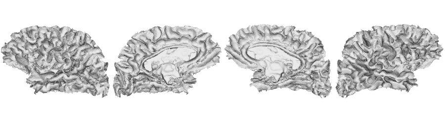
`fsLR-32k`: Middle surface 

# Native fsLR-32k midsurface
fsLR32k_mid_lh = read_surface(dir_surf+subjectID+'_hemi-L_space-nativepro_surf-fsLR-32k_label-midthickness.surf.gii', itype='gii')
fsLR32k_mid_rh = read_surface(dir_surf+subjectID+'_hemi-R_space-nativepro_surf-fsLR-32k_label-midthickness.surf.gii', itype='gii')

# Plot the surface
plot_hemispheres(fsLR32k_mid_lh, fsLR32k_mid_rh, size=(900, 250), zoom=1.25, embed_nb=True, interactive=False, share='both',
                 nan_color=(0, 0, 0, 1), color_range=(-1,1), cmap='Greys', transparent_bg=False)

# Load fsLR-32k middle surfaces for left and right hemispheres.
f32k.mid.lh <- read.fs.surface(filepath = paste0(dir_surf, subjectID,'_hemi-L_space-nativepro_surf-fsLR-32k_label-midthickness.surf.gii') )
f32k.mid.rh <- read.fs.surface(filepath = paste0(dir_surf, subjectID,'_hemi-R_space-nativepro_surf-fsLR-32k_label-midthickness.surf.gii') )

# Prepare and plot the surfaces for visualization.
cml = coloredmesh.from.preloaded.data(f32k.mid.lh, morph_data = rnorm(nrow(f32k.mid.lh$vertices),5,1), makecmap_options = list('colFn'=grays) )
cmr = coloredmesh.from.preloaded.data(f32k.mid.rh, morph_data = rnorm(nrow(f32k.mid.rh$vertices),5,1), makecmap_options = list('colFn'=grays) )
f32k.mid <- brainviews(views = 't4', coloredmeshes=list('lh'=cml, 'rh'=cmr), draw_colorbar = FALSE,
           rglactions = list('trans_fun'=limit_fun(-1, 1), 'no_vis'=T))
plot_surface(f32k.mid, 'fsLR-32k mid')

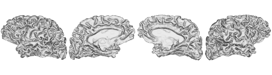
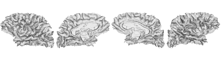
`fsLR-32k`: White matter surface 

# Native fsLR-32k white matter
fsLR32k_wm_lh = read_surface(dir_surf+subjectID+'_hemi-L_space-nativepro_surf-fsLR-32k_label-white.surf.gii', itype='gii')
fsLR32k_wm_rh = read_surface(dir_surf+subjectID+'_hemi-R_space-nativepro_surf-fsLR-32k_label-white.surf.gii', itype='gii')

# Plot the surface
plot_hemispheres(fsLR32k_wm_lh, fsLR32k_wm_lh, size=(900, 250), zoom=1.25, embed_nb=True, interactive=False, share='both',
                 nan_color=(0, 0, 0, 1), color_range=(1.5, 4), cmap='Greys', transparent_bg=False)

# Load fsLR-32k white surfaces for left and right hemispheres.
f32k.wm.lh <- read.fs.surface(filepath = paste0(dir_surf, subjectID,'_hemi-L_space-nativepro_surf-fsLR-32k_label-white.surf.gii') )
f32k.wm.rh <- read.fs.surface(filepath = paste0(dir_surf, subjectID,'_hemi-R_space-nativepro_surf-fsLR-32k_label-white.surf.gii') )

# Prepare and plot the surfaces for visualization.
cml <- coloredmesh.from.preloaded.data(f32k.wm.lh, morph_data = rnorm(nrow(f32k.wm.lh$vertices),5,1), makecmap_options = list('colFn'=grays) )
cmr <- coloredmesh.from.preloaded.data(f32k.wm.rh, morph_data = rnorm(nrow(f32k.wm.rh$vertices),5,1), makecmap_options = list('colFn'=grays) )
f32k.wm <- brainviews(views = 't4', coloredmeshes=list('lh'=cml, 'rh'=cmr), draw_colorbar = FALSE,
           rglactions = list('trans_fun'=limit_fun(-1, 1), 'no_vis'=T))
plot_surface(f32k.wm, 'fsLR-32k white')

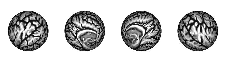
Native sphere 

# Native sphere
sph_lh = read_surface(dir_surf+subjectID+'_hemi-L_surf-fsnative_label-sphere.surf.gii', itype='gii')
sph_rh = read_surface(dir_surf+subjectID+'_hemi-R_surf-fsnative_label-sphere.surf.gii', itype='gii')

# Plot the surface
plot_hemispheres(sph_lh, sph_rh, array_name=cv, size=(900, 250), zoom=1.25, embed_nb=True, interactive=False, share='both',
                 nan_color=(0, 0, 0, 1), color_range=(-0.2, 0.2), cmap="gray", transparent_bg=False)

# Load native sphere surfaces for left and right hemispheres.
sph.lh <- read.fs.surface(filepath = paste0(dir_surf, subjectID,'_hemi-L_surf-fsnative_label-sphere.surf.gii'))
sph.rh <- read.fs.surface(filepath = paste0(dir_surf, subjectID,'_hemi-R_surf-fsnative_label-sphere.surf.gii'))

# Prepare colored meshes with curvature data.
cml <- coloredmesh.from.preloaded.data(sph.lh, morph_data = lfc(readgii(cv.lh)$data$unknown), hemi = 'lh', makecmap_options = list('colFn'=bw))
cmr <- coloredmesh.from.preloaded.data(sph.rh, morph_data = lfc(readgii(cv.rh)$data$unknown), hemi = 'rh', makecmap_options = list('colFn'=bw))
sph.nat <- brainviews(views = 't4', coloredmeshes=list('lh'=cml, 'rh'=cmr), rglactions = list('no_vis'=T))

# Display the native sphere surface with mapped curvature data.
plot_surface(sph.nat, 'Native sphere curvature [1/mm]')

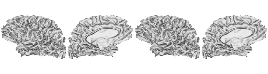
Superficial White Matter (SWM) in `fsnative` surface 

The superficial white matter surfaces are generated across 3 different surface layer from the white mater to 1, 2 and 3mm deeps. Then each quantitative map from /maps is resample from fsnative to fsaverage5, fsLR-32k and fsLR-5k. In this example we will only plot the native surfaces.

SWM Surfaces 

# Function to load and plot each SWM surfaces
def plot_swm(mm='1'):
    # SWM fsnative 1mm
    swm_lh = read_surface(f'{dir_surf}{subjectID}_hemi-L_surf-fsnative_label-swm{mm}.0mm.surf.gii', itype='gii')
    swm_rh = read_surface(f'{dir_surf}{subjectID}_hemi-R_surf-fsnative_label-swm{mm}.0mm.surf.gii', itype='gii')

    # Plot the surface
    fig = plot_hemispheres(swm_lh, swm_rh, size=(900, 250), zoom=1.25, embed_nb=True, interactive=False, share='both',
                     nan_color=(0, 0, 0, 1), color_range=(1.5, 4), cmap='Greys', transparent_bg=False)
    return(fig)

# Function to visualize SWM at varying depths (1mm, 2mm, 3mm).
mesh_swm <- function(mm = '1') {

  # Load SWM surface data for specified depth for both hemispheres.
  f32k.swm.lh <- read.fs.surface(filepath = paste0(dir_surf, subjectID,'_hemi-L_surf-fsnative_label-swm',mm,'.0mm.surf.gii') )
  f32k.swm.rh <- read.fs.surface(filepath = paste0(dir_surf, subjectID,'_hemi-R_surf-fsnative_label-swm',mm,'.0mm.surf.gii') )

  # Generate colored meshes using random morphometric data for visualization.
  cml = coloredmesh.from.preloaded.data(f32k.swm.lh, morph_data = rnorm(nrow(f32k.swm.lh$vertices),5,1), makecmap_options = list('colFn'=grays) )
  cmr = coloredmesh.from.preloaded.data(f32k.swm.rh, morph_data = rnorm(nrow(f32k.swm.rh$vertices),5,1), makecmap_options = list('colFn'=grays) )
  bv <- brainviews(views = 't4', coloredmeshes=list('lh'=cml, 'rh'=cmr), draw_colorbar = FALSE,
             rglactions = list('trans_fun'=limit_fun(-1, 1), 'no_vis'=T))
  return(bv)
}

SWM 1mm 

# SWM 1mm
plot_swm(mm='1')

# SWM 1mm
plot_surface(mesh_swm('1'), 'Superficial white matter 1mm depth')

SWM 2mm 

# SWM 2mm
plot_swm(mm='2')

# SWM 2mm
plot_surface(mesh_swm('2'), 'Superficial white matter 2mm depth')

SWM 3mm 

# SWM 3mm
plot_swm(mm='3')

# SWM 3mm
plot_surface(mesh_swm('3'), 'Superficial white matter 3mm depth')

`/maps`: `fsnative`, `fsaverage5`, `fsLR-32k` and `fsLR-5k`

Each file map with the extension func.gii corresponds to the data map from a NIFTI image at a certain deep.
The deep from where it was mapped is in the name after the string label-.
The hemisphere is either L for left or R for right.
The surface will match the number of points of the surface that corresponds that file map. The options are: fsnative, fsLR-32k, fsLR-5k and fsaverage5.

Note ❕

For example the file below corresponds to the left native surface mapped from midthicknes of the T1map nifti image: sub-001_hemi-L_surf-fsnative_label-midthickness_T1map.func.gii

The maps on the surfaces fsnative, fsLR-32k, fsLR-5k, can be plot on their native surface or on the standard surface (regular or inflated).

Warning

There is NO inherent smoothing applied to the map. If the user desires smoothing, they should customize it according to their preferences and requirements.

def load_qmri(qmri='', surf='fsLR-32k'):
    '''
    This function loads the qMRI intensity maps from midthickness surface
    '''
    # List the files
    files_lh = sorted(glob.glob(f"{dir_maps}/*_hemi-L_surf-{surf}_label-midthickness_{qmri}.func.gii"))
    files_rh = sorted(glob.glob(f"{dir_maps}/*_hemi-R_surf-{surf}_label-midthickness_{qmri}.func.gii"))

    # Load map data
    surf_map=np.concatenate((nib.load(files_lh[0]).darrays[0].data, nib.load(files_rh[0]).darrays[0].data), axis=0)

    return(surf_map)

def plot_qmri(qmri='',  surf='fsLR-32k', label='pial', cmap='rocket', rq=(0.15, 0.95)):
    '''
    This function plots the qMRI intensity maps on the pial surface
    '''
    # Load the data
    map_surf = load_qmri(qmri, surf)
    print('Number of vertices: ' + str(map_surf.shape[0]))

    # Load the surfaces
    surf_lh=read_surface(f'{dir_surf}/{subjectID}_hemi-L_space-nativepro_surf-{surf}_label-{label}.surf.gii', itype='gii')
    surf_rh=read_surface(f'{dir_surf}/{subjectID}_hemi-R_space-nativepro_surf-{surf}_label-{label}.surf.gii', itype='gii')

    # Color range based in the quantiles
    crange=(np.quantile(map_surf, rq[0]), np.quantile(map_surf, rq[1]))

    # Plot the group T1map intensitites
    fig = plot_hemispheres(surf_lh, surf_rh, array_name=map_surf, size=(900, 250), color_bar='bottom', zoom=1.25, embed_nb=True, interactive=False, share='both',
                     nan_color=(0, 0, 0, 1), cmap=cmap, color_range=crange, transparent_bg=False, screenshot = False)
    return(fig)

# Function to aggregate qMRI surface data paths for a given type and surface.
surf_qmri <- function(qmri = '', surf = 'fsLR-32k') {

  # Compile file paths for qMRI data across hemispheres.
  files_lh <- paste0(dir_maps, subjectID, '_hemi-L_surf-', surf, '_label-midthickness_', qmri, '.func.gii')
  files_rh <- paste0(dir_maps, subjectID, '_hemi-R_surf-', surf, '_label-midthickness_', qmri, '.func.gii')

  # Combine left and right hemisphere data into a single array.
  surf_map <- c(readgii(files_lh)$data, readgii(files_rh)$data)

  return(surf_map)
}

# Function to visualize qMRI data on a specified brain surface.
mesh_qmri <- function(qmri = '', surf = 'fsLR-32k', label = 'pial', rq = c(0.15, 0.95), cmap = inferno) {

  # Retrieve qMRI data mapped to specified surface.
  map_surf <- surf_qmri(qmri, surf)

  # Load associated surface data for visualization.
  surf.lh <- read.fs.surface(filepath = paste0(dir_surf, '/', subjectID, '_hemi-L_space-nativepro_surf-', surf, '_label-', label, '.surf.gii' ) )
  surf.rh <- read.fs.surface(filepath = paste0(dir_surf, '/', subjectID, '_hemi-R_space-nativepro_surf-', surf, '_label-', label, '.surf.gii' ) )

  # Determine data range for color mapping based on specified quantiles.
  crange <- quantile(c(map_surf[[1]], map_surf[[2]]), probs = rq)

  # Set the color limits
  lf= limit_fun(crange[1], crange[2])

  # Apply color mapping based on the data range.
  cml = coloredmesh.from.preloaded.data(surf.lh, morph_data = lf(map_surf[[1]]), makecmap_options = list('colFn'=cmap) )
  cmr = coloredmesh.from.preloaded.data(surf.rh, morph_data = lf(map_surf[[2]]), makecmap_options = list('colFn'=cmap) )

  # Generate and return the visual representation.
  return(brainviews(views = 't4', coloredmeshes=list('lh'=cml, 'rh'=cmr), draw_colorbar = FALSE, rglactions = list('trans_fun'=limit_fun(-1, 1), 'no_vis'=T)))
}

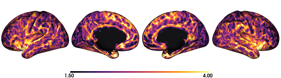
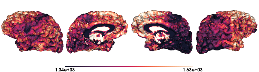
T1map on `fsnative`

# Plot of T1map on fsnative
plot_qmri('T1map', 'fsnative')

# T1 map on fsnative surface
plot_surface(mesh_qmri(qmri = 'T1map', surf = 'fsnative'))

# Plot of T1map on fsnative
plot_qmri('T1map', 'fsnative')

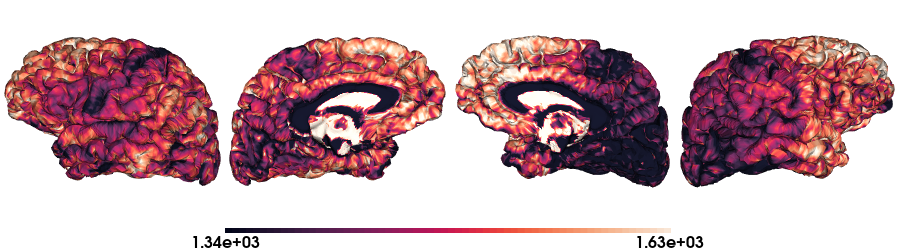
T1map on `fsaverage5` native 

# Plot of T1map on fsaverage5
plot_qmri('T1map', 'fsaverage5')

# T1 map on fsaverage5 surface
plot_surface(mesh_qmri(qmri = 'T1map', surf = 'fsaverage5'))

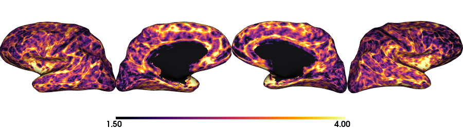
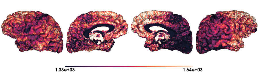
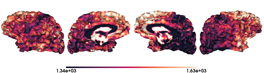
T1map on `fsLR-32k` native 

# Plot of T1map on fsLR-32k
plot_qmri('T1map', 'fsLR-32k')

# T1 map on fsLR-32k surface
plot_surface(mesh_qmri(qmri = 'T1map', surf = 'fsLR-32k'))

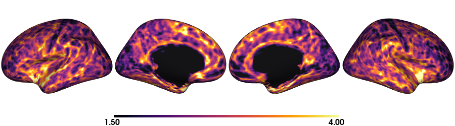
T1map on `fsLR-5k` native 

# Plot of T1map on fsLR-5k
plot_qmri('T1map', 'fsLR-5k')

# T1 map on fsLR-5k surface
plot_surface(mesh_qmri(qmri = 'T1map', surf = 'fsLR-5k'))

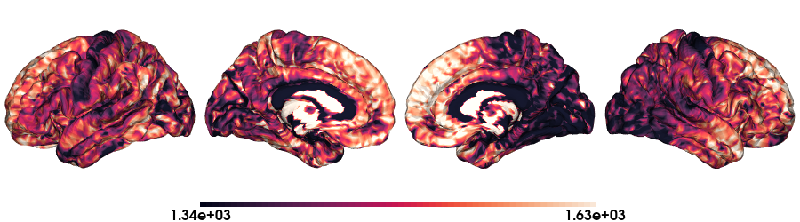
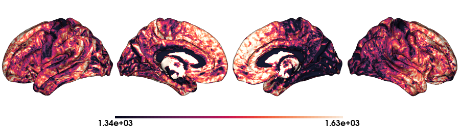
`/maps`: `fsaverage5`, `fsLR-32k` and `fsLR-5k` on standard 

T1map on `fsaverage5` standard 

# Load the T1map data on fsaverage5
map_data = load_qmri('T1map', 'fsaverage5')

# Color range based in the quantiles
crange=(np.quantile(map_data, 0.15), np.quantile(map_data, 0.95))

# Plot data on standard surface
plot_hemispheres(fs5_lh, fs5_rh, array_name=map_data, size=(900, 250), color_bar='bottom', zoom=1.25, embed_nb=True, interactive=False, share='both',
                         nan_color=(0, 0, 0, 1), color_range=crange, cmap="rocket", transparent_bg=False)

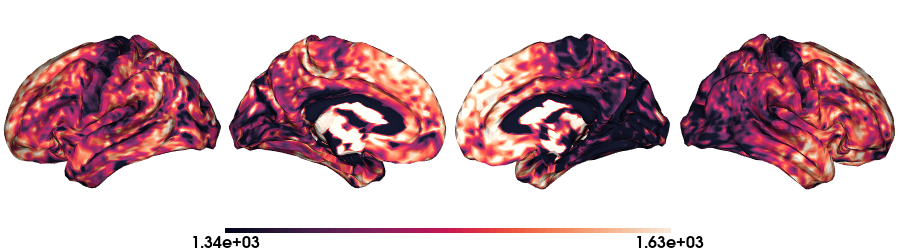
T1map on `fsLR-32k` stardard 

# Load the T1map data on fsLR-32k
map_data = load_qmri('T1map', 'fsLR-32k')

# Plot data on standard surface
plot_hemispheres(f32k_lh, f32k_rh, array_name=map_data, size=(900, 250), color_bar='bottom', zoom=1.25, embed_nb=True, interactive=False, share='both',
                         nan_color=(0, 0, 0, 1), color_range=crange, cmap="rocket", transparent_bg=False)

T1map on `fsLR-5k` stardard 

# Load the T1map data on fsLR-5k
map_data = load_qmri('T1map', 'fsLR-5k')

# Plot data on standard surface
plot_hemispheres(f5k_lh, f5k_rh, array_name=map_data, size=(900, 250), color_bar='bottom', zoom=1.25, embed_nb=True, interactive=False, share='both',
                         nan_color=(0, 0, 0, 1), color_range=crange, cmap="rocket", transparent_bg=False)

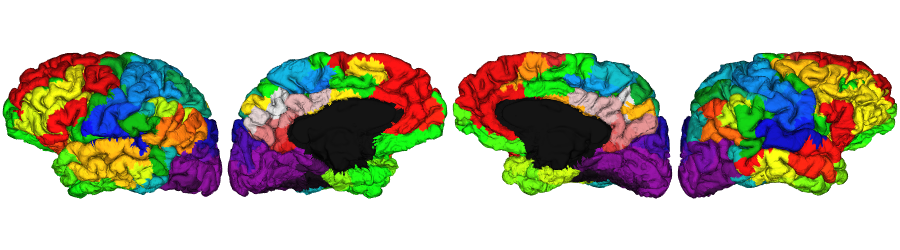
Atlas labels on surface 

All the native surface labels generated by micapipe are stored inside the subject’s freesurfer directory.

Schaefer-400 labels 

# Load annotation file
annot = 'schaefer-400'
annot_lh= dir_FS + '/label/lh.' + annot + '_mics.annot'
annot_rh= dir_FS + '/label/rh.' + annot + '_mics.annot'
label = np.concatenate((nib.freesurfer.read_annot(annot_lh)[0], nib.freesurfer.read_annot(annot_rh)[0]), axis=0)

# plot labels on surface
plot_hemispheres(pial_lh, pial_rh, array_name=label, size=(900, 250), zoom=1.25, embed_nb=True, interactive=False, share='both',
                 nan_color=(0, 0, 0, 1), cmap='nipy_spectral', transparent_bg=False)

# Generate and visualize Schaefer-400 labels on the pial surface.
schaefer.400 <- vis.subject.annot('freesurfer/', subjectID, 'schaefer-400_mics', 'both', surface='pial',
                           views=NULL, rglactions = list('no_vis'=T))

plot_surface(schaefer.400, 'Schaefer-400')

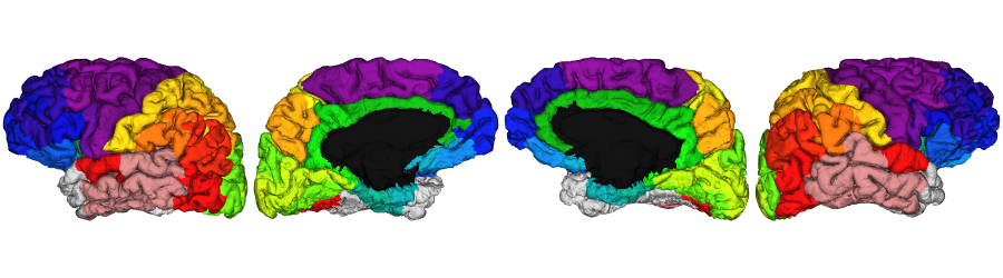
Extra: Economo labels 

# Load annotation file
annot = 'economo'
annot_lh= dir_FS + '/label/lh.' + annot + '_mics.annot'
annot_rh= dir_FS + '/label/rh.' + annot + '_mics.annot'
label = np.concatenate((nib.freesurfer.read_annot(annot_lh)[0], nib.freesurfer.read_annot(annot_rh)[0]), axis=0)

# plot labels on surface
plot_hemispheres(pial_lh, pial_rh, array_name=label, size=(900, 250), zoom=1.25, embed_nb=True, interactive=False, share='both',
                 nan_color=(0, 0, 0, 1), cmap='nipy_spectral', transparent_bg=False)

# Generate and visualize Economo cortical labels on the pial surface.
economo <- vis.subject.annot('freesurfer/', subjectID, 'economo_mics', 'both', surface='pial',
                           views=NULL, rglactions = list('no_vis'=T))
plot_surface(economo, 'economo', img_only=TRUE)

Download code examples: Surfaces 

Python Jupyter notebook: 'tutorial_surface_visualization.ipynb'

Python source code: 'tutorial_surface_visualization.py'

R source code: 'tutorial_surface_visualization.R'