Main output matrices

This section describes where are the main connectomes generated by the pipeline, and how you can visualize them using python or R. All the outputs are BIDS conform and stored under their correspondent directory (e.g. anat, func dwi). This example will use the subject HC001, session 01 from the MICs dataset, and all paths will be relative to the subject directory or out/micapipe/sub-HC001_ses01/

Organization of the outputs

If you are inside the out directory, where the pipeline’s outputs are stored, two folders can be found inside, one for each pipeline used. For this dataset, the main structure should look like this:

out
├── freesurfer
└── micapipe

Inside the directory called micapipe a new directory will be created for each subject processed, defined with the string sub- and the subject’s identification. Three more files can be found:

pipeline-description.json: This file contains the last version of micapipe that was used and, the inherited information about the dataset used.

micapipe_processed_sub.csv: This is a csv table stores information about the modules processed by subject, date of last run and the status (complete or incomplete).

micapipe_progress.html: This file is generated with the option -QC, it is a html that eases the visualization of the processed subjects.

The subject list is truncated to the first three subjects

micapipe/
├── micapipe_processed_sub.csv
├── pipeline-description.json
├── micapipe_progress.html
├── sub-HC001
├── sub-HC002
├── sub-HC003
...

Inside each subject’s directory you’ll find the session folders, unless you have a single session and you don’t specify the ses- in your dataset. Six main directories are inside each subject folder: anat, dwi, func, logs, QC and xfm. The connectomes are stored in four main directories:

Geodesic distance connectome: anat/surfaces/geo_dist

Microstructural profile connectome: anat/surfaces/micro_profiles

Structural connectome (DWI): dwi/connectomes

Functional connectome (rsfMRI): func/surfaces

The structure of the subject HC001 directories is shown below:

sub-HC001/
└── ses-01
    ├── anat
    │   ├── first                # fsl first outputs
    │   ├── surfaces
    │   │   ├── conte69          # conte69 surfaces
    │   │   ├── geo_dist         # Geodesic distance connectomes
    │   │   ├── micro_profiles   # MPC connectomes and surfaces
    │   │   └── morphology       # Thickness and curvature surfaces
    │   └── volumetric           # Parceellations in nativepro space
    ├── dwi
    │   ├── connectomes          # DWI connectomes
    │   └── eddy                 # fsl eddy outputs
    ├── func
    │   ├── surfaces             # rsfMRI surfaces and connectomes
    │   └── volumetric           # rsfMRI volumes
    ├── logs                     # log files
    ├── QC
    │   ├── eddy_QC              # fsl eddy_quad outputs
    │   └── png                  # PNG images for QC
    └── xfm                      # Trasnformation matrices and warpfields

In the following examples we’ll focus on how to load and visualize the connectome matrices of a single subject. Even though we generate up to 18 connectomes, we’ll only use the atlas schaefer-400 for visualization and practicality purposes. All the paths are relative to the subject’s directory, which in our case is out/micapipe/sub-HC001/ses-01.

This example uses the packages nilearn, numpy and matplotlib for python, and RColorBrewer and viridis for R. The first step in both languages is to set the environment:

# Set the environment
import os
import numpy as np
from nilearn import plotting
import matplotlib as plt

# Set the working directory to the 'out' directory
os.chdir("~/out") # <<<<<<<<<<<< CHANGE THIS PATH

# This variable will be different for each subject
subjectID='sub-HC001_ses-01'           # <<<<<<<<<<<< CHANGE THIS SUBJECT's ID
subjectDir='micapipe/sub-HC001/ses-01' # <<<<<<<<<<<< CHANGE THIS SUBJECT's DIRECTORY

# Here we define the atlas
atlas='schaefer-400' # <<<<<<<<<<<< CHANGE THIS ATLAS

# Set the environment
require("RColorBrewer")
require("viridis")

# Set the working directory to your subjec's directory
setwd("out/micapipe/sub-HC001/ses-01")

# This variable will be different for each subject
subjectID <- 'sub-HC001_ses-01'

# Here we define the atlas
atlas <- 'schaefer-400'

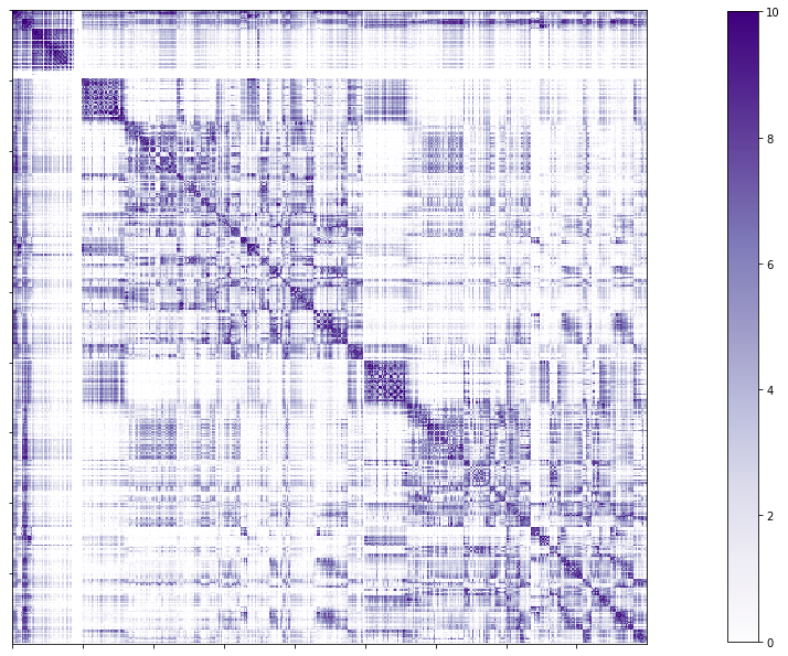
Structural connectome

Structural connectomes are stored in the dwi/connectomes directory. Three main connectomes are generated per atlas, and are identified with a specific string:

cor-connectome: Contains only cortical nodes.
sub-connectome: This connectome contains the cortical nodes and subcortical structures.
full-connectome: Full connectome has cerebellar, subcortical and cortical nodes.

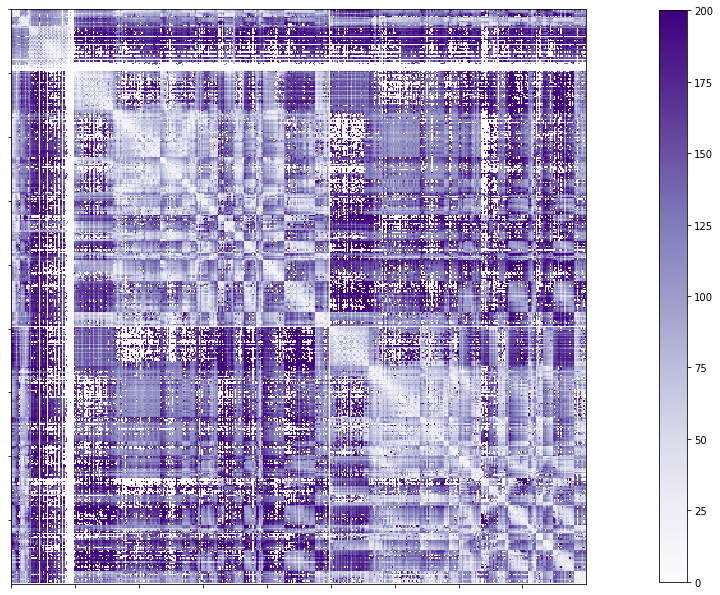
Additionally, the edge lengths of each of the previous connectomes are stored in different files with the string edgeLengths.

A total of 6 files per atlas are generated by the pipeline, the main organization is shown below:

dwi/connectomes/
├── sub-HC005_ses-01_space-dwi_atlas-schaefer-400_desc-iFOD2-40M-SIFT2_cor-connectome.txt
├── sub-HC005_ses-01_space-dwi_atlas-schaefer-400_desc-iFOD2-40M-SIFT2_cor-edgeLengths.txt
├── sub-HC005_ses-01_space-dwi_atlas-schaefer-400_desc-iFOD2-40M-SIFT2_full-connectome.txt
├── sub-HC005_ses-01_space-dwi_atlas-schaefer-400_desc-iFOD2-40M-SIFT2_full-edgeLengths.txt
├── sub-HC005_ses-01_space-dwi_atlas-schaefer-400_desc-iFOD2-40M-SIFT2_sub-connectome.txt
└── sub-HC005_ses-01_space-dwi_atlas-schaefer-400_desc-iFOD2-40M-SIFT2_sub-edgeLengths.txt

Full structural connectome

# Set the path to the the structural cortical connectome
cnt_sc_cor = 'dwi/connectomes/' + subjectID + '_space-dwi_atlas-' + atlas + '_desc-iFOD2-40M-SIFT2_full-connectome.txt'

# Load the cortical connectome
mtx_sc = np.loadtxt(cnt_sc_cor, dtype=np.float, delimiter=' ')

# Fill the lower triangle of the matrix
mtx_scSym = np.triu(mtx_sc,1)+mtx_sc.T

# Plot the log matrix
corr_plot = plotting.plot_matrix(np.log(mtx_scSym), figure=(10, 10), labels=None, cmap='Purples', vmin=0, vmax=10)

# Set the path to the the structural cortical connectome
cnt_sc_cor <- paste0('dwi/connectomes/', subjectID, '_space-dwi_atlas-', atlas, '_desc-iFOD2-40M-SIFT2_full-connectome.txt')

# Load the cortical connectome
mtx_sc <- as.matrix(read.csv(cnt_sc_cor, sep=" ", header <- FALSE,))

# Fill the lower triangle of the matrix
mtx_sc[lower.tri(mtx_sc)] <- t(mtx_sc)[lower.tri(mtx_sc)]

# Plot the log matrix
image(log(mtx_sc), axes=FALSE, main=paste0("SC ", atlas), col=brewer.pal(9, "Purples"))

Full structural connectome edge lengths

# Set the path to the the structural cortical connectome
cnt_sc_EL = cnt_sc_cor='dwi/connectomes/' + subjectID + '_space-dwi_atlas-' + atlas + '_desc-iFOD2-40M-SIFT2_full-edgeLengths.txt'

# Load the cortical connectome
mtx_scEL = np.loadtxt(cnt_sc_EL, dtype=np.float, delimiter=' ')

# Fill the lower triangle of the matrix
mtx_scELSym = np.triu(mtx_scEL,1)+mtx_sc.T

# Plot the log matrix
corr_plot = plotting.plot_matrix(mtx_scELSym, figure=(10, 10), labels=None, cmap='Purples', vmin=0, vmax=10)

# Set the path to the the structural cortical connectome
cnt_sc_EL <- paste0('dwi/connectomes/', subjectID, '_space-dwi_atlas-', atlas, '_desc-iFOD2-40M-SIFT2_full-edgeLengths.txt')

# Load the cortical connectome
mtx_scEL <- as.matrix(read.csv(cnt_sc_EL, sep=" ", header=FALSE,))

# Fill the lower triangle of the matrix
mtx_scEL[lower.tri(mtx_scEL)] <- t(mtx_scEL)[lower.tri(mtx_scEL)]

# Plot the log matrix
image(log(mtx_scEL), axes=FALSE, main=paste0("SC ", atlas), col=brewer.pal(9, "Purples"))

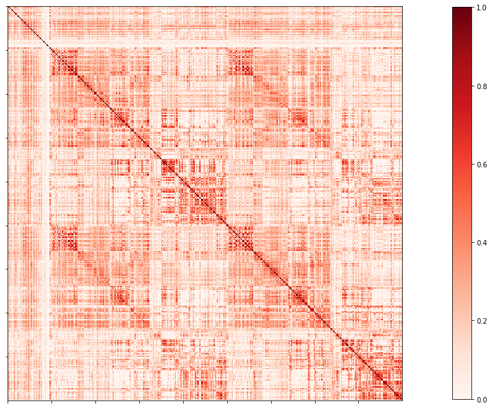
Resting state Functional connectome

For each atlas, two files are generated: the functional connectome (desc-FC.txt) and the time-series of that atlas (desc-timeseries.txt).

func/surfaces/
├── sub-HC005_ses-01_rsfmri_space-fsnative_atlas-schaefer-400_desc-FC.txt
└── sub-HC005_ses-01_rsfmri_space-fsnative_atlas-schaefer-400_desc-timeseries.txt

# Set the path to the the functional connectome
cnt_fs = 'func/surfaces/' + subjectID + '_rsfmri_space-fsnative_atlas-' + atlas + '_desc-FC.txt'

# Load the connectome
mtx_fs = np.loadtxt(cnt_fs, dtype=np.float, delimiter=' ')

# Fill the lower triangle of the matrix
mtx_fcSym = np.triu(mtx_fs,1)+mtx_fs.T

# Plot the matrix
corr_plot = plotting.plot_matrix(mtx_fcSym, figure=(10, 10), labels=None, cmap='Reds')

# Set the path to the the functional connectome
cnt_fs <- paste0('func/surfaces/', subjectID, '_rsfmri_space-fsnative_atlas-', atlas, '_desc-FC.txt')

# Load the cortical connectome
mtx_fs <- as.matrix(read.csv(cnt_fs, sep=" ", header=FALSE))

# Fill the lower triangle of the matrix
mtx_fs[lower.tri(mtx_fs)] <- t(mtx_fs)[lower.tri(mtx_fs)]

# Plot the matrix
image(mtx_fs, axes=FALSE, main=paste0("FC ", atlas), col=brewer.pal(9, "Reds"))

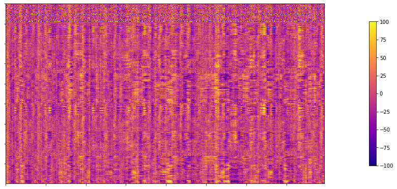
Resting state time series

# Set the path to the the time series file
cnt_time = 'func/surfaces/' + subjectID + '_rsfmri_space-fsnative_atlas-' + atlas + '_desc-timeseries.txt'

# Load the time series
mtx_time = np.loadtxt(cnt_time, dtype=np.float, delimiter=' ')

# Plot as a matrix
corr_plot = plotting.plot_matrix(mtx_time.T, figure=(12, 5), labels=None, cmap='Reds')

# Set the path to the the time series file
cnt_time <- paste0('func/surfaces/', subjectID, '_rsfmri_space-fsnative_atlas-', atlas, '_desc-timeseries.txt')

# Load the time series
mtx_time <- as.matrix(read.csv(cnt_time, sep=" ", header=FALSE))

# Plot as a matrix
image(mtx_time, axes=FALSE, main=paste0("Time series ", atlas), col=plasma(64))

MPC connectome

For each atlas, two files are generated: the microstructural profile covariance connectome (desc-MPC.txt) and the intensity profile of that atlas (desc-intensity_profiles.txt).

anat/surfaces/micro_profiles/
├── sub-HC005_ses-01_space-fsnative_atlas-schaefer-400_desc-intensity_profiles.txt
└── sub-HC005_ses-01_space-fsnative_atlas-schaefer-400_desc-MPC.txt

# Set the path to the the MPC cortical connectome
cnt_mpc = 'anat/surfaces/micro_profiles/' + subjectID + '_space-fsnative_atlas-' + atlas + '_desc-MPC.txt'

# Load the cortical connectome
mtx_mpc = np.loadtxt(cnt_mpc, dtype=np.float, delimiter=' ')

# Fill the lower triangle of the matrix
mtx_mpcSym = np.triu(mtx_mpc,1)+mtx_mpc.T

# Plot the log matrix
corr_plot = plotting.plot_matrix(mtx_mpcSym, figure=(10, 10), labels=None, cmap='Greens')

# Set the path to the the MPC cortical connectome
cnt_mpc <- paste0('anat/surfaces/micro_profiles/', subjectID, '_space-fsnative_atlas-', atlas, '_desc-MPC.txt')

# Load the cortical connectome
mtx_mpc <- as.matrix(read.csv(cnt_mpc, sep=" ", header=FALSE))

# Fill the lower triangle of the matrix
mtx_mpc[lower.tri(mtx_mpc)] <- t(mtx_mpc)[lower.tri(mtx_mpc)]

# Plot the matrix
image(mtx_mpc, axes=FALSE, main=paste0("MPC ", atlas), col=brewer.pal(9, "Greens"))

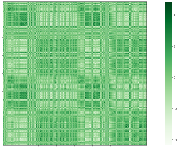
Intensity profiles

# Set the path to the the time series file
cnt_int = 'anat/surfaces/micro_profiles/' + subjectID + '_space-fsnative_atlas-' + atlas + '_desc-intensity_profiles.txt'

# Load the time series
mtx_int = np.loadtxt(cnt_int, dtype=np.float, delimiter=' ')

# Plot as a matrix
corr_plot = plotting.plot_matrix(mtx_int, figure=(20,10), labels=None, cmap='Greens', colorbar=False)

# Set the path to the the time series file
cnt_int <- paste0('anat/surfaces/micro_profiles/', subjectID, '_space-fsnative_atlas-', atlas, '_desc-intensity_profiles.txt')

# Load the time series
mtx_int <- as.matrix(read.csv(cnt_int, sep=" ", header=FALSE))

# Plot as a matrix
image(mtx_int, axes=FALSE, main=paste0("Intensity profiles", atlas), col=brewer.pal(9, "Greens"))

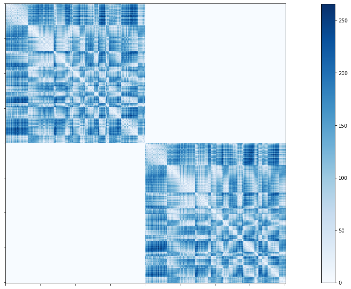
Geodesic distance connectome

Only one file per atlas is generated by this module:

anat/surfaces/geo_dist/
└── sub-HC005_ses-01_space-fsnative_atlas-schaefer-400_GD.txt

# Set the path to the the geodesic distance connectome
cnt_gd = 'anat/surfaces/geo_dist/' + subjectID + '_space-fsnative_atlas-' + atlas + '_GD.txt'

# Load the cortical connectome
mtx_gd = np.loadtxt(cnt_gd, dtype=np.float, delimiter=' ')

# Plot the log matrix
corr_plot = plotting.plot_matrix(mtx_gd, figure=(10, 10), labels=None, cmap='Blues')

# Set the path to the the geodesic distance connectome
cnt_gd <- paste0('anat/surfaces/geo_dist/', subjectID, '_space-fsnative_atlas-', atlas, '_GD.txt')

# Load the cortical connectome
mtx_gd <- as.matrix(read.csv(cnt_gd, sep=" ", header=FALSE))

# Plot the matrix
image(mtx_gd, axes=FALSE, main=paste0("GD ", atlas), col=brewer.pal(9, "Blues"))

Download code examples: matrices

Python Jupyter notebook: 'tutorial_main_output_matrices.ipynb'

Python source code: 'tutorial_main_output_matrices.py'

R source code: 'tutorial_main_output_matrices.R'