Building gradients
Table of Contents
This section describes how to generate macroscale gradient mapping from the output matrices of micapipe. The matrices are the same as in the Main output matrices tutorial.
For this tutorial we will map each modality of a single subject using BrainSpace, a python based library.
For further information about how to use BrainSpace and macroscale gradient mapping and analysis of neuroimaging and connectome level data visit their documentation here: BrainSpace documentation
Additionally the libraries os, numpy, nibabel and nibabel will be used.
As in previous examples, we will use the subject HC001, session 01 from the MICs dataset, and all paths will be relative to the subject directory or out/micapipe_v0.2.0/sub-HC001_ses01/ and the atlas schaefer-400.
In this tutorial we will only plot the first 3 components of the diffusion map embedding (aka gradients).
python environment
The first step is to set the python environment and all the variables relative to the subject you’re interested to visualize.
 1# Set the environment
 2import os
 3import glob
 4import numpy as np
 5import nibabel as nib
 6from brainspace.plotting import plot_hemispheres
 7from brainspace.mesh.mesh_io import read_surface
 8from brainspace.datasets import load_conte69
 9from brainspace.gradient import GradientMaps
10from brainspace.utils.parcellation import map_to_labels
11import matplotlib.pyplot as plt
12
13# Set the working directory to the 'out' directory
14out='/data_/mica3/BIDS_MICs/derivatives'
15os.chdir(out)     # <<<<<<<<<<<< CHANGE THIS PATH
16
17# This variable will be different for each subject
18sub='HC001' # <<<<<<<<<<<< CHANGE THIS SUBJECT's ID
19ses='01'    # <<<<<<<<<<<< CHANGE THIS SUBJECT's SESSION
20subjectID=f'sub-{sub}_ses-{ses}'
21subjectDir=f'micapipe_v0.2.0/sub-{sub}/ses-{ses}'
22
23# Here we define the atlas
24atlas='schaefer-400' # <<<<<<<<<<<< CHANGE THIS ATLAS
25
26# Path to MICAPIPE from global enviroment
27micapipe=os.popen("echo $MICAPIPE").read()[:-1] # <<<<<<<<<<<< CHANGE THIS PATH
Loading the surfaces
 1 # Load fsLR-32k
 2 f32k_lh = read_surface(f'{micapipe}/surfaces/fsLR-32k.L.surf.gii', itype='gii')
 3 f32k_rh = read_surface(f'{micapipe}/surfaces/fsLR-32k.R.surf.gii', itype='gii')
 4
 5 # Load fsaverage5
 6 fs5_lh = read_surface(f'{micapipe}/surfaces/fsaverage5/surf/lh.pial', itype='fs')
 7 fs5_rh = read_surface(f'{micapipe}/surfaces/fsaverage5/surf/rh.pial', itype='fs')
 8
 9 # Load LEFT annotation file in fsaverage5
10 annot_lh_fs5= nib.freesurfer.read_annot(f'{micapipe}/parcellations/lh.{atlas}_mics.annot')
11
12 # Unique number of labels of a given atlas
13 Ndim = max(np.unique(annot_lh_fs5[0]))
14
15 # Load RIGHT annotation file in fsaverage5
16 annot_rh_fs5= nib.freesurfer.read_annot(f'{micapipe}/parcellations/rh.{atlas}_mics.annot')[0]+Ndim
17
18 # replace with 0 the medial wall of the right labels
19 annot_rh_fs5 = np.where(annot_rh_fs5==Ndim, 0, annot_rh_fs5)
20
21 # fsaverage5 labels
22 labels_fs5 = np.concatenate((annot_lh_fs5[0], annot_rh_fs5), axis=0)
23
24 # Mask of the medial wall on fsaverage 5
25 mask_fs5 = labels_fs5 != 0
26
27 # Read label for fsLR-32k
28 labels_f32k = np.loadtxt(open(f'{micapipe}/parcellations/{atlas}_conte69.csv'), dtype=int)
29
30 # mask of the medial wall
31 mask_f32k = labels_f32k != 0
Global variables
1# Number of gradients to calculate
2Ngrad=10
3
4# Number of gradients to plot
5Nplot=3
6
7# Labels for plotting based on Nplot
8labels=['G'+str(x) for x in list(range(1,Nplot+1))]
Gradients from atlas based connectomes: single subject
Geodesic distance
Load and slice the GD matrix
1 # Set the path to the the geodesic distance connectome
2 gd_file = f'{subjectDir}/dist/{subjectID}_atlas-{atlas}_GD.shape.gii'
3
4 # Load the cortical connectome
5 mtx_gd = nib.load(gd_file).darrays[0].data
6
7 # Remove the Mediall Wall
8 mtx_gd = np.delete(np.delete(mtx_gd, 0, axis=0), 0, axis=1)
9 GD = np.delete(np.delete(mtx_gd, Ndim, axis=0), Ndim, axis=1)
Calculate the GD gradients
1 # GD Left hemi
2 gm_GD_L = GradientMaps(n_components=Ngrad, random_state=None, approach='dm', kernel='normalized_angle')
3 gm_GD_L.fit(GD[0:Ndim, 0:Ndim], sparsity=0.8)
4
5 # GD Right hemi
6 gm_GD_R = GradientMaps(n_components=Ngrad, alignment='procrustes', kernel='normalized_angle'); # align right hemi to left hemi
7 gm_GD_R.fit(GD[Ndim:Ndim*2, Ndim:Ndim*2], sparsity=0.85, reference=gm_GD_L.gradients_)
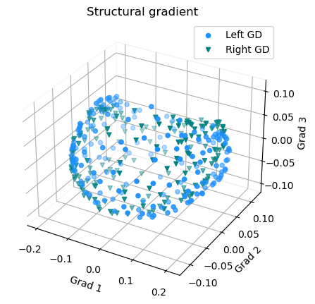
Plot the GD gradients
 1 # plot the gradients
 2 g1=gm_GD_L.gradients_[:, 0]
 3 g2=gm_GD_L.gradients_[:, 1]
 4 g3=gm_GD_L.gradients_[:, 2]
 5
 6 # plot the gradients
 7 g1R=gm_GD_R.aligned_[:, 0]
 8 g2R=gm_GD_R.aligned_[:, 1]
 9 g3R=gm_GD_R.aligned_[:, 2]
10
11 # Creating figure
12 fig = plt.figure(figsize=(7, 5))
13 ax = fig.add_subplot(111, projection="3d")
14
15 # Creating plot
16 ax.scatter3D(g1, g2, g3, color = 'dodgerblue')
17 ax.scatter3D(g1R, g2R, g3R, color = 'teal', marker='v')
18 plt.title("Structural gradient")
19 ax.legend(['Left GD', 'Right GD'])
20
21 ax.set_xlabel('Grad 1')
22 ax.set_ylabel('Grad 2')
23 ax.set_zlabel('Grad 3')
24
25 # Remove the outer box lines
26 ax.xaxis.pane.fill = False
27 ax.yaxis.pane.fill = False
28 ax.zaxis.pane.fill = False
29
30 # Show plot
31 plt.show()
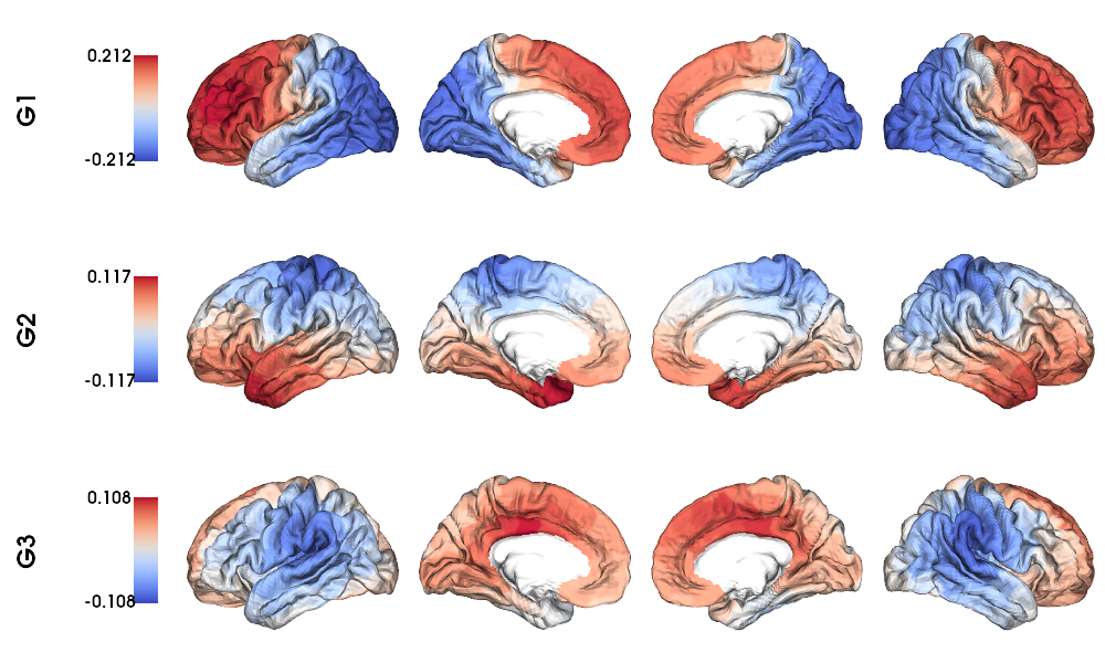
GD gradients on fsaverage5 surface
 1 # Left and right gradients concatenated
 2 GD_gradients = np.concatenate((gm_GD_L.gradients_, gm_GD_R.aligned_), axis=0)
 3
 4 # Map gradients to original parcels
 5 grad = [None] * Nplot
 6 for i, g in enumerate(GD_gradients.T[0:Nplot,:]):
 7     grad[i] = map_to_labels(g, labels_fs5,  fill=np.nan, mask=mask_fs5)
 8
 9 # Plot Gradients RdYlBu
10 plot_hemispheres(fs5_lh, fs5_rh, array_name=grad, size=(1000, 600), cmap='coolwarm',
11                  embed_nb=True,  label_text={'left':labels}, color_bar='left',
12                  zoom=1.25, nan_color=(1, 1, 1, 1), color_range = 'sym' )
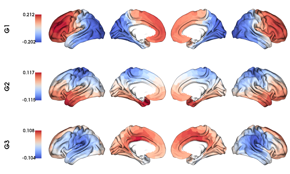
GD gradients to fsLR-32k surface
1 # Map gradients to original parcels
2 grad = [None] * Nplot
3 for i, g in enumerate(GD_gradients.T[0:Nplot,:]):
4     grad[i] = map_to_labels(g, labels_f32k, fill=np.nan, mask=mask_f32k)
5
6 # Plot Gradients
7 plot_hemispheres(f32k_lh, f32k_rh, array_name=grad, size=(1000, 600), cmap='coolwarm',
8                  embed_nb=True,  label_text={'left':labels}, color_bar='left',
9                  zoom=1.25, nan_color=(1, 1, 1, 1))
Structural gradients
Load and slice the structural matrix
 1 # Set the path to the the structural cortical connectome
 2 sc_file = f'{subjectDir}/dwi/connectomes/{subjectID}_space-dwi_atlas-{atlas}_desc-iFOD2-40M-SIFT2_full-connectome.shape.gii'
 3
 4 # Load the cortical connectome
 5 mtx_sc = nib.load(sc_file).darrays[0].data
 6
 7 # Fill the lower triangle of the matrix
 8 mtx_sc = np.log(np.triu(mtx_sc,1)+mtx_sc.T)
 9 mtx_sc[np.isneginf(mtx_sc)] = 0
10
11 # Slice the connectome to use only cortical nodes
12 SC = mtx_sc[49:, 49:]
13 SC = np.delete(np.delete(SC, 200, axis=0), 200, axis=1)
Calculate the structural gradients
1 # SC Left hemi
2 gm_SC_L = GradientMaps(n_components=Ngrad, random_state=None, approach='dm', kernel='normalized_angle')
3 gm_SC_L.fit(SC[0:Ndim, 0:Ndim], sparsity=0.9)
4
5 # SC Right hemi
6 gm_SC_R = GradientMaps(n_components=Ngrad, alignment='procrustes', kernel='normalized_angle'); # align right hemi to left hemi
7 gm_SC_R.fit(SC[Ndim:Ndim*2, Ndim:Ndim*2], sparsity=0.9, reference=gm_SC_L.gradients_)
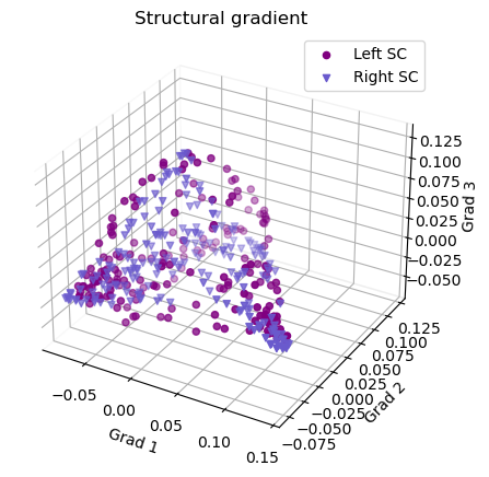
Plot the structural gradients
 1 # plot the left gradients
 2 g1=gm_SC_L.gradients_[:, 0]
 3 g2=gm_SC_L.gradients_[:, 1]
 4 g3=gm_SC_L.gradients_[:, 2]
 5
 6 # plot the right gradients
 7 g1R=gm_SC_R.aligned_[:, 0]
 8 g2R=gm_SC_R.aligned_[:, 1]
 9 g3R=gm_SC_R.aligned_[:, 2]
10
11 # Creating figure
12 fig = plt.figure(figsize=(7, 5))
13 ax = fig.add_subplot(111, projection="3d")
14
15 # Creating plot
16 ax.scatter3D(g1, g2, g3, color = 'purple')
17 ax.scatter3D(g1R, g2R, g3R, color = 'slateblue', marker='v')
18 plt.title("Structural gradient")
19 ax.legend(['Left SC', 'Right SC'])
20
21 ax.set_xlabel('Grad 1')
22 ax.set_ylabel('Grad 2')
23 ax.set_zlabel('Grad 3')
24
25 # Remove the outer box lines
26 ax.xaxis.pane.fill = False
27 ax.yaxis.pane.fill = False
28 ax.zaxis.pane.fill = False
29
30 # Show plot
31 plt.show()
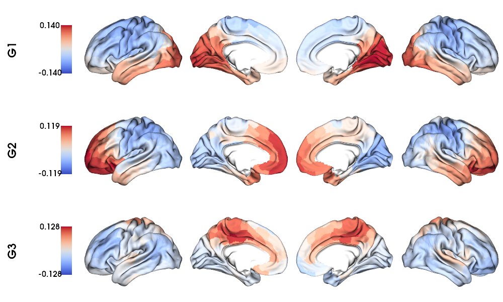
Structural gradients on fsLR-32k surface
 1 # Left and right gradients concatenated
 2 SC_gradients = np.concatenate((gm_SC_L.gradients_, gm_SC_R.aligned_), axis=0)
 3
 4 # Map gradients to original parcels
 5 grad = [None] * Nplot
 6 for i, g in enumerate(SC_gradients.T[0:Nplot,:]):
 7 grad[i] = map_to_labels(g, labels_f32k, fill=np.nan, mask=mask_f32k)
 8
 9 # Plot Gradients
10 plot_hemispheres(f32k_lh, f32k_rh, array_name=grad, size=(1000, 600), cmap='coolwarm',
11      embed_nb=True,  label_text={'left':labels}, color_bar='left',
12      zoom=1.25, nan_color=(1, 1, 1, 1), color_range = 'sym' )
Functional gradients
Load and slice the functional matrix
 1 # acquisitions
 2 func_acq='desc-se_task-rest_acq-AP_bold'
 3 fc_file = f'{subjectDir}/func/{func_acq}/surf/{subjectID}_surf-fsLR-32k_atlas-{atlas}_desc-FC.shape.gii'
 4
 5 # Load the cortical connectome
 6 mtx_fs = nib.load(fc_file).darrays[0].data
 7
 8 # slice the matrix to keep only the cortical ROIs
 9 FC = mtx_fs[49:, 49:]
10 #FC = np.delete(np.delete(FC, Ndim, axis=0), Ndim, axis=1)
11
12 # Fischer transformation
13 FCz = np.arctanh(FC)
14
15 # replace inf with 0
16 FCz[~np.isfinite(FCz)] = 0
17
18 # Mirror the matrix
19 FCz = np.triu(FCz,1)+FCz.T
Calculate the functional gradients
1 # Calculate the gradients
2 gm = GradientMaps(n_components=Ngrad, random_state=None, approach='dm', kernel='normalized_angle')
3 gm.fit(FCz, sparsity=0.85)
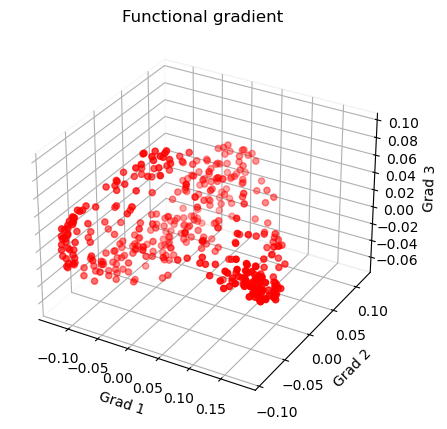
Plot the functional gradients
 1 # Plot the gradients
 2 g1 = gm.gradients_[:, 0]
 3 g2 = gm.gradients_[:, 1]
 4 g3 = gm.gradients_[:, 2]
 5
 6 # Creating figure
 7 fig = plt.figure(figsize=(7, 5))
 8 ax = fig.add_subplot(111, projection="3d")
 9
10 # Creating plot
11 ax.scatter3D(g1, g2, g3, color='red')
12 plt.title("Functional gradient")
13
14 ax.set_xlabel('Grad 1')
15 ax.set_ylabel('Grad 2')
16 ax.set_zlabel('Grad 3')
17
18 # Remove the outer box lines
19 ax.xaxis.pane.fill = False
20 ax.yaxis.pane.fill = False
21 ax.zaxis.pane.fill = False
22
23 # Show plot
24 plt.show()
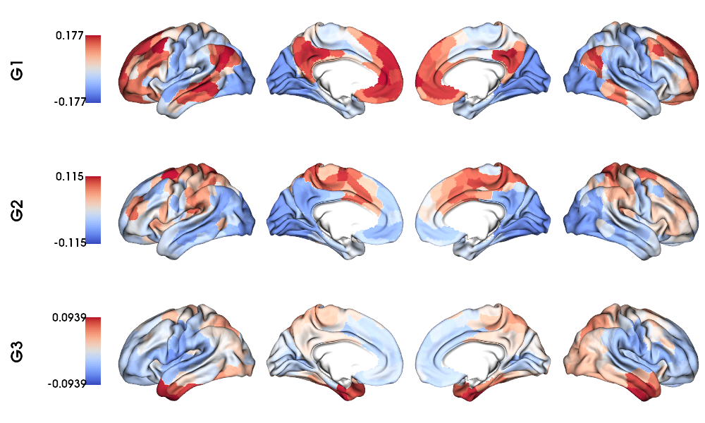
Functional gradients on fsLR-32k surface
1 # Map gradients to original parcels
2 grad = [None] * Nplot
3 for i, g in enumerate(gm.gradients_.T[0:Nplot,:]):
4     grad[i] = map_to_labels(g, labels_f32k, fill=np.nan, mask=mask_f32k)
5
6 # Plot Gradients coolwarm
7 plot_hemispheres(f32k_lh, f32k_rh, array_name=grad, size=(1000, 600), cmap='coolwarm',
8                  embed_nb=True,  label_text={'left':labels}, color_bar='left',
9                  zoom=1.25, nan_color=(1, 1, 1, 1), color_range = 'sym')
MPC gradients
Function to load MPC
 1 # Define a function to load and process the MPC matrices
 2 def load_mpc(File, Ndim):
 3     """Loads and process a MPC"""
 4
 5     # Load file
 6     mpc = nib.load(File).darrays[0].data
 7
 8     # Mirror the lower triangle
 9     mpc = np.triu(mpc,1)+mpc.T
10
11     # Replace infinite values with epsilon
12     mpc[~np.isfinite(mpc)] = np.finfo(float).eps
13
14     # Replace 0 with epsilon
15     mpc[mpc==0] = np.finfo(float).eps
16
17     # Remove the medial wall
18     mpc = np.delete(np.delete(mpc, 0, axis=0), 0, axis=1)
19     mpc = np.delete(np.delete(mpc, Ndim, axis=0), Ndim, axis=1)
20
21     # retun the MPC
22     return(mpc)
List and load the MPC matrix
1 # Set the path to the the MPC cortical connectome
2 mpc_acq='acq-T1map'
3 mpc_file = f'{subjectDir}/mpc/{mpc_acq}/{subjectID}_atlas-{atlas}_desc-MPC.shape.gii'
4
5 # Load the cortical connectome
6 mpc = load_mpc(mpc_file, Ndim)
Calculate the MPC gradients
1 # Calculate the gradients
2 gm = GradientMaps(n_components=Ngrad, random_state=None, approach='dm', kernel='normalized_angle')
3 gm.fit(mpc, sparsity=0)
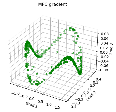
Plot the MPC gradients
 1 # Plot the gradients
 2 g1 = gm.gradients_[:, 0]
 3 g2 = gm.gradients_[:, 1]
 4 g3 = gm.gradients_[:, 2]
 5
 6 # Creating figure
 7 fig = plt.figure(figsize=(7, 5))
 8 ax = fig.add_subplot(111, projection="3d")
 9
10 # Creating plot
11 ax.scatter3D(g1, g2, g3, color = 'green')
12 plt.title("MPC gradient")
13
14 ax.set_xlabel('Grad 1')
15 ax.set_ylabel('Grad 2')
16 ax.set_zlabel('Grad 3')
17
18 # Remove the outer box lines
19 ax.xaxis.pane.fill = False
20 ax.yaxis.pane.fill = False
21 ax.zaxis.pane.fill = False
22
23 # Show plot
24 plt.show()
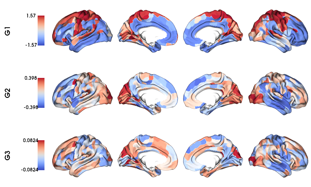
MPC gradients on fsLR-32k surface
1 # Map gradients to original parcels
2 grad = [None] * Nplot
3 for i, g in enumerate(gm.gradients_.T[0:Nplot,:]):
4     grad[i] = map_to_labels(g, labels_f32k, fill=np.nan, mask=mask_f32k)
5
6 # Plot Gradients
7 plot_hemispheres(f32k_lh, f32k_rh, array_name=grad, size=(1000, 600), cmap='coolwarm',
8                  embed_nb=True,  label_text={'left':labels}, color_bar='left',
9                  zoom=1.25, nan_color=(1, 1, 1, 1), color_range = 'sym' )
Load all matrices from a dataset processed
Start by generating a list of files using regular expressions for matrices with a consistent structure. Specifically, we’ll focus on loading the
T1map MPCconnectome data forschaefer-400from the MPC directory.Create an empty three-dimensional array with dimensions
{ROI * ROI * subjects}.Load each matrix iteratively and populate the array with the data.
Once the array is populated, perform computations on it. In this case, we’ll calculate the group mean connectome.
Use the group mean connectome to compute the group mean diffusion map for the
T1map MPC.Finally, visualize the results by plotting the first three gradients (eigen vectors) of the group mean diffusion map on a surface
fsLR-32k.
MPC gradients: ALL subjects mean
Load all the MPC matrices
 1 # MPC T1map acquisition
 2 mpc_acq='T1map'
 3
 4 # 1. List all the matrices from all subjects
 5 mpc_files = sorted(glob.glob(f'micapipe_v0.2.0/sub-PX*/ses-*/mpc/acq-{mpc_acq}/*_atlas-{atlas}_desc-MPC.shape.gii'))
 6 N = len(mpc_files)
 7 print(f"Number of subjects's MPC: {N}")
 8
 9 # 2. Empty 3D array to load the data
10 mpc_all=np.empty([Ndim*2, Ndim*2, len(mpc_files)], dtype=float)
11
12 # 3. Load all the  MPC matrices
13 for i, f in enumerate(mpc_files):
14     mpc_all[:,:,i] = load_mpc(f, Ndim)
15
16 # Print the shape of the 3D-array: {roi * roi * subjects}
17 mpc_all.shape
Calculate the mean group MPC gradients
1 # 4. Mean group MPC across all subjects (z-axis)
2 mpc_all_mean = np.mean(mpc_all, axis=2)
3
4 # Calculate the gradients
5 gm = GradientMaps(n_components=Ngrad, random_state=None, approach='dm', kernel='normalized_angle')
6 gm.fit(mpc_all_mean, sparsity=0)
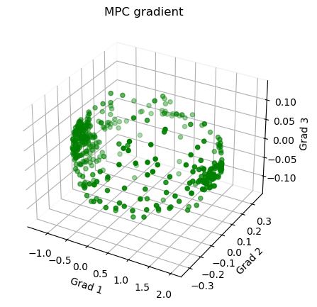
Plot the mean group MPC gradients
 1 # Plot the gradients
 2 g1 = gm.gradients_[:, 0]
 3 g2 = gm.gradients_[:, 1]
 4 g3 = gm.gradients_[:, 2]
 5
 6 # Creating figure
 7 fig = plt.figure(figsize=(7, 5))
 8 ax = fig.add_subplot(111, projection="3d")
 9
10 # Creating plot
11 ax.scatter3D(g1, g2, g3, color = 'green')
12 plt.title("MPC gradient")
13
14 ax.set_xlabel('Grad 1')
15 ax.set_ylabel('Grad 2')
16 ax.set_zlabel('Grad 3')
17
18 # Remove the outer box lines
19 ax.xaxis.pane.fill = False
20 ax.yaxis.pane.fill = False
21 ax.zaxis.pane.fill = False
22
23 # Show plot
24 plt.show()
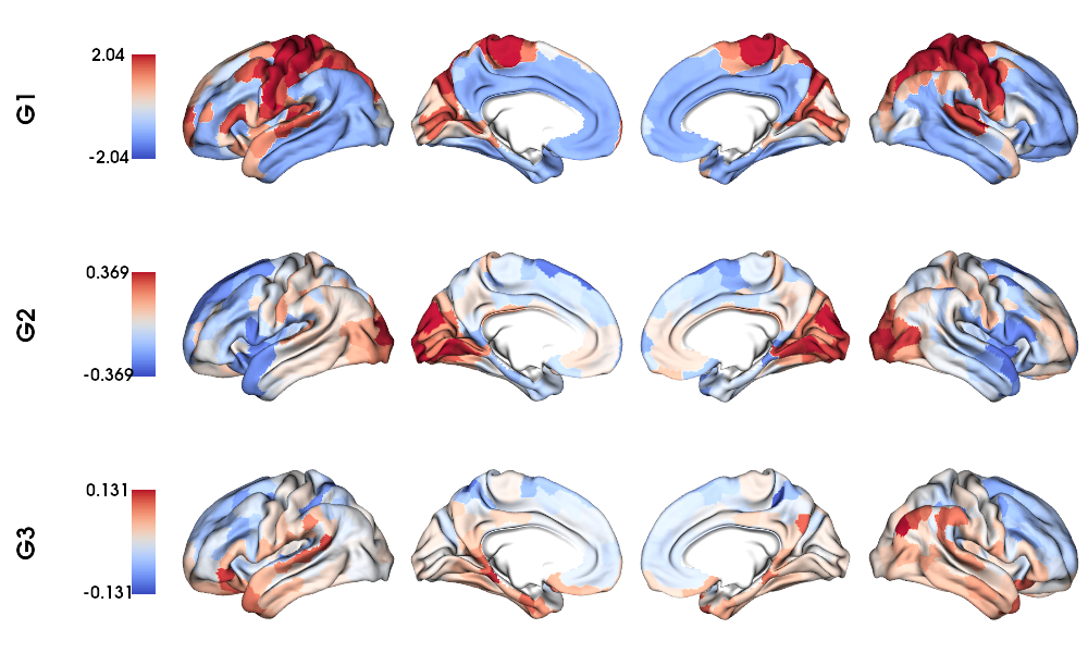
Mean group MPC gradients on fsLR-32k surface
1 # Map gradients to original parcels
2 grad = [None] * Nplot
3 for i, g in enumerate(gm.gradients_.T[0:Nplot,:]):
4     grad[i] = map_to_labels(g, labels_f32k, fill=np.nan, mask=mask_f32k)
5
6 # Plot Gradients
7 plot_hemispheres(f32k_lh, f32k_rh, array_name=grad, size=(1000, 600), cmap='coolwarm',
8                  embed_nb=True,  label_text={'left':labels}, color_bar='left',
9                  zoom=1.25, nan_color=(1, 1, 1, 1), color_range = 'sym' )
fsLR-5k gradients
Environment
 1 # Set the environment
 2 import os
 3 import glob
 4 import numpy as np
 5 import nibabel as nib
 6 from brainspace.plotting import plot_hemispheres
 7 from brainspace.mesh.mesh_io import read_surface
 8 from brainspace.datasets import load_conte69
 9 from brainspace.gradient import GradientMaps
10 from brainspace.utils.parcellation import map_to_labels
11 import matplotlib.pyplot as plt
12
13 # Set the working directory to the 'out' directory
14 out='/data_/mica3/BIDS_MICs/derivatives'  # <<<<<<<<<<<< CHANGE THIS PATH
15 os.chdir(f'{out}/micapipe_v0.2.0')
16
17 # This variable will be different for each subject
18 sub='HC001' # <<<<<<<<<<<< CHANGE THIS SUBJECT's ID
19 ses='01'    # <<<<<<<<<<<< CHANGE THIS SUBJECT's SESSION
20 subjectID=f'sub-{sub}_ses-{ses}'
21 subjectDir=f'micapipe_v0.2.0/sub-{sub}/ses-{ses}'
22
23 # Path to MICAPIPE from global enviroment
24 micapipe=os.popen("echo $MICAPIPE").read()[:-1] # <<<<<<<<<<<< CHANGE THIS PATH
Load the surfaces
1 # Load fsLR-5k inflated surface
2 micapipe='/data_/mica1/01_programs/micapipe-v0.2.0'
3 f5k_lhi = read_surface(micapipe + '/surfaces/fsLR-5k.L.inflated.surf.gii', itype='gii')
4 f5k_rhi = read_surface(micapipe + '/surfaces/fsLR-5k.R.inflated.surf.gii', itype='gii')
5
6 # fsLR-5k mask
7 mask_lh = nib.load(micapipe + '/surfaces/fsLR-5k.L.mask.shape.gii').darrays[0].data
8 mask_rh = nib.load(micapipe + '/surfaces/fsLR-5k.R.mask.shape.gii').darrays[0].data
9 mask_5k = np.concatenate((mask_lh, mask_rh), axis=0)
Functions to load fsLR-5k connectomes
 1 # Define functions to load GD, SC, FC and MPC fsLR-32k
 2 def load_mpc(File):
 3     """Loads and process a MPC"""
 4
 5     # Load file
 6     mpc = nib.load(File).darrays[0].data
 7
 8     # Mirror the lower triangle
 9     mpc = np.triu(mpc,1)+mpc.T
10
11     # Replace infinite values with epsilon
12     mpc[~np.isfinite(mpc)] = np.finfo(float).eps
13
14     # Replace 0 with epsilon
15     mpc[mpc==0] = np.finfo(float).eps
16
17     # retun the MPC
18     return(mpc)
19
20 def load_gd(File):
21     """Loads and process a GD"""
22
23     # load the matrix
24     mtx_gd = nib.load(File).darrays[0].data
25
26     return mtx_gd
27
28 def load_fc(File):
29     """Loads and process a functional connectome"""
30
31     # load the matrix
32     FC = nib.load(File).darrays[0].data
33
34     # Fisher transform
35     FCz = np.arctanh(FC)
36
37     # replace inf with 0
38     FCz[~np.isfinite(FCz)] = 0
39
40     # Mirror the matrix
41     FCz = np.triu(FCz,1)+FCz.T
42     return FCz
43
44 def load_sc(File):
45     """Loads and process a structura connectome"""
46
47     # load the matrix
48     mtx_sc = nib.load(File).darrays[0].data
49
50     # Mirror the matrix
51     mtx_sc = np.triu(mtx_sc,1)+mtx_sc.T
52
53     return mtx_sc
Functions to calculate fsLR-5k diffusion maps
 1 # Gradients aka eigen vector of the diffusion map embedding
 2 def fslr5k_dm_lr(mtx, mask_5k, Ngrad=3, log=True, S=0):
 3     """
 4     Create the gradients from the SC or GD matrices.
 5     Use log=False for GD gradients
 6     """
 7     if log != True:
 8         mtx_log = mtx
 9     else:
10         # log transform the connectome
11         mtx_log = np.log(mtx)
12
13     # Replace NaN with 0
14     mtx_log[np.isnan(mtx_log)] = 0
15
16     # Replace negative infinite with 0
17     mtx_log[np.isneginf(mtx_log)] = 0
18
19     # Replace infinite with 0
20     mtx_log[~np.isfinite(mtx_log)] = 0
21
22     # replace 0 values with almost 0
23     mtx_log[mtx_log==0] = np.finfo(float).eps
24
25     # Left and right mask
26     indx_L = np.where(mask_5k[0:4842]==1)[0]
27     indx_R = np.where(mask_5k[4842:9684]==1)[0]
28
29     # Left and right SC
30     mtx_L = mtx_log[0:4842, 0:4842]
31     mtx_R = mtx_log[4842:9684, 4842:9684]
32
33     # Slice the matrix
34     mtx_L_masked = mtx_L[indx_L, :]
35     mtx_L_masked = mtx_L_masked[:, indx_L]
36     mtx_R_masked = mtx_R[indx_R, :]
37     mtx_R_masked = mtx_R_masked[:, indx_R]
38
39     # mtx Left hemi
40     mtx_L = GradientMaps(n_components=Ngrad, random_state=None, approach='dm', kernel='normalized_angle')
41     mtx_L.fit(mtx_L_masked, sparsity=S)
42
43     # mtx Right hemi
44     mtx_R = GradientMaps(n_components=Ngrad, alignment='procrustes', kernel='normalized_angle'); # align right hemi to left hemi
45     mtx_R.fit(mtx_R_masked, sparsity=S, reference=mtx_L.gradients_)
46
47     # Left and right gradients concatenated
48     mtx_gradients = np.concatenate((mtx_L.gradients_, mtx_R.aligned_), axis=0)
49
50     # Boolean mask
51     mask_surf = mask_5k != 0
52
53     # Get the index of the non medial wall regions
54     indx = np.where(mask_5k==1)[0]
55
56     # Map gradients to surface
57     grad = [None] * Ngrad
58     for i, g in enumerate(mtx_gradients.T[0:Ngrad,:]):
59         # create a new array filled with NaN values
60         g_nan = np.full(mask_surf.shape, np.nan)
61         g_nan[indx] = g
62         grad[i] = g_nan
63
64     return(mtx_gradients, grad)
65
66 def fslr5k_dm(mtx, mask, Ngrad=3, S=0.9):
67     """Create the gradients from the MPC matrix
68         S=sparcity, by default is 0.9
69     """
70     # Cleanup before diffusion embeding
71     mtx[~np.isfinite(mtx)] = 0
72     mtx[np.isnan(mtx)] = 0
73     mtx[mtx==0] = np.finfo(float).eps
74
75     # Get the index of the non medial wall regions
76     indx = np.where(mask==1)[0]
77
78     # Slice the matrix
79     mtx_masked = mtx[indx, :]
80     mtx_masked = mtx_masked[:, indx]
81
82     # Calculate the gradients
83     gm = GradientMaps(n_components=Ngrad, random_state=None, approach='dm', kernel='normalized_angle')
84     gm.fit(mtx_masked, sparsity=S)
85
86     # Map gradients to surface
87     grad = [None] * Ngrad
88
89     # Boolean mask
90     mask_surf = mask != 0
91
92     for i, g in enumerate(gm.gradients_.T[0:Ngrad,:]):
93
94         # create a new array filled with NaN values
95         g_nan = np.full(mask_surf.shape, np.nan)
96         g_nan[indx] = g
97         grad[i] = g_nan
98
99     return(gm, grad)
Global variables
 1 # Number of vertices of the fsLR-5k matrices (per hemisphere)
 2 N5k = 9684
 3
 4 # Number of gradients to calculate
 5 Ngrad=10
 6
 7 # Number of gradients to plot
 8 Nplot=3
 9
10 # Labels for plotting based on Nplot
11 labels=['G'+str(x) for x in list(range(1,Nplot+1))]
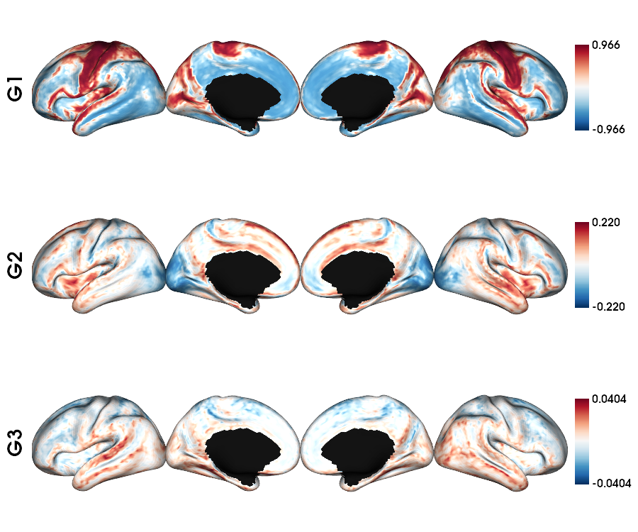
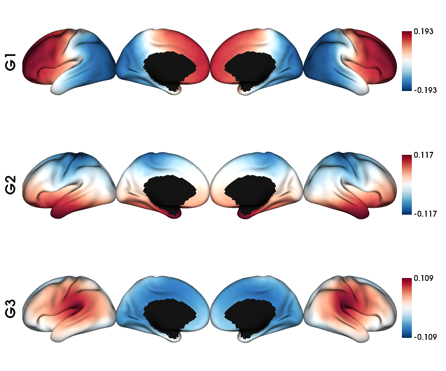
Geodesic distance: single subject fsLR-5k
 1 # List the file
 2 gd_file = glob.glob(f"sub-{sub}/ses-{ses}/dist/*_surf-fsLR-5k_GD.shape.gii")
 3
 4 # Loads the GD fsLR-5k matrix
 5 gd_5k = load_gd(gd_file[0])
 6
 7 # Calculate the gradients
 8 gd_dm, grad = fslr5k_dm_lr(gd_5k, mask_5k, Ngrad=Ngrad, log=False, S=0.85)
 9
10 # plot the gradients
11 plot_hemispheres(f5k_lhi, f5k_rhi, array_name=grad[0:Nplot], cmap='RdBu_r', nan_color=(0, 0, 0, 1),
12   zoom=1.3, size=(900, 750), embed_nb=True, color_range='sym',
13   color_bar='right', label_text={'left': labels})
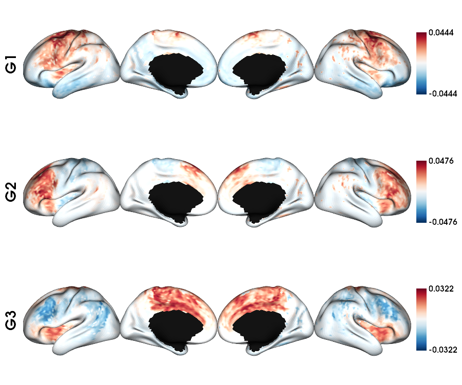
Structual connectome: single subject fsLR-5k
 1 # List the file
 2 sc_file = sorted(glob.glob(f"sub-{sub}/ses-{ses}/dwi/connectomes/*_surf-fsLR-5k_desc-iFOD2-40M-SIFT2_full-connectome.shape.gii"))
 3
 4 # Loads the SC fsLR-5k matrix
 5 sc_5k = load_sc(sc_file[0])
 6
 7 # Calculate the gradients
 8 sc_dm, grad = fslr5k_dm_lr(sc_5k, mask_5k, Ngrad=Ngrad, log=False, S=0.9)
 9
10 # PLot the gradients (G2-G4)
11 plot_hemispheres(f5k_lhi, f5k_rhi, array_name=grad[1:Nplot+1], cmap='RdBu_r', nan_color=(0, 0, 0, 1),
12   zoom=1.3, size=(900, 750), embed_nb=True, color_range='sym',
13   color_bar='right', label_text={'left': labels})
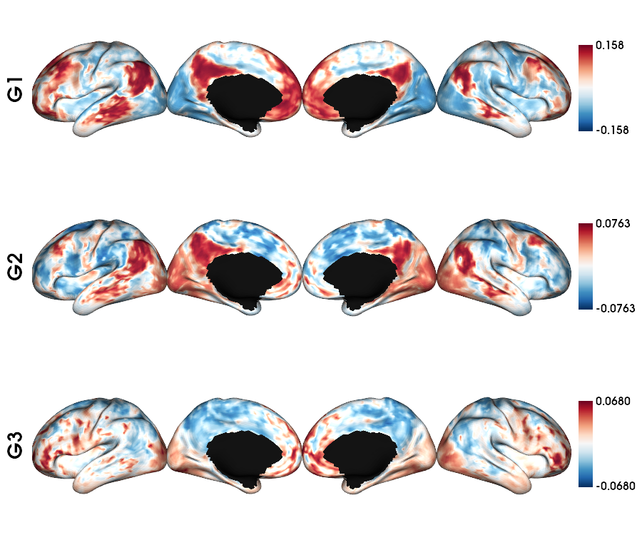
Functional connectome: single subject fsLR-5k
 1 # List the file
 2 func_acq='desc-se_task-rest_acq-AP_bold'
 3 fc_file = sorted(glob.glob(f"sub-{sub}/ses-{ses}/func/{func_acq}/surf/*_surf-fsLR-5k_desc-FC.shape.gii"))
 4
 5 # Loads the FC fsLR-5k matrix
 6 fc_5k = load_fc(fc_file[0])
 7
 8 # Calculate the gradients
 9 fc_dm, grad = fslr5k_dm(fc_5k, mask_5k, Ngrad=Ngrad, S=0.9)
10
11 # plot the gradients
12 plot_hemispheres(f5k_lhi, f5k_rhi, array_name=grad[0:Nplot], cmap='RdBu_r', nan_color=(0, 0, 0, 1),
13   zoom=1.3, size=(900, 750), embed_nb=True, color_range='sym',
14   color_bar='right', label_text={'left': labels})
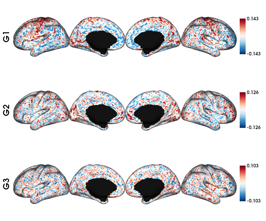
MPC T1map: single subject fsLR-5k
 1 # MPC T1map acquisition and file
 2 mpc_acq='T1map'
 3 mpc_file = sorted(glob.glob(f"sub-{sub}/ses-{ses}/mpc/acq-{mpc_acq}/*surf-fsLR-5k_desc-MPC.shape.gii"))
 4
 5 # Loads the MPC fsLR-5k matrix
 6 mpc_5k = load_mpc(mpc_file[0])
 7
 8 # Calculate the gradients (diffusion map)
 9 mpc_dm, grad = fslr5k_dm(mpc_5k, mask_5k, Ngrad=Ngrad, Smooth=True, S=0.9)
10
11 # Plot the gradients
12 plot_hemispheres(f5k_lhi, f5k_rhi, array_name=grad[0:Nplot], cmap='RdBu_r', nan_color=(0, 0, 0, 1),
13   zoom=1.3, size=(900, 750), embed_nb=True, color_range='sym',
14   color_bar='right', label_text={'left': labels})
MPC T1map: ALL subjects fsLR-5k
Load all matrices from a dataset processed
Start by generating a list of files using regular expressions for matrices with a consistent structure. Specifically, we’ll focus on loading the
T1map MPCconnectome data forfsLR-5kfrom the MPC directory.Create an empty three-dimensional array with dimensions
{ROI * ROI * vertices}.Load each matrix iteratively and populate the array with the data.
Once the array is populated, perform computations on it. In this case, we’ll calculate the group mean connectome.
Use the group mean connectome to compute the group mean diffusion map for the
T1map MPC.Finally, visualize the results by plotting the first three gradients (eigen vectors) of the group mean diffusion map on a surface
fsLR-5k.
 1 # MPC T1map acquisition
 2 mpc_acq='T1map'
 3
 4 # List all the matrices from all subjects
 5 mpc_file = sorted(glob.glob(f"sub-PX*/ses-01/mpc/acq-{mpc_acq}/*surf-fsLR-5k_desc-MPC.shape.gii"))
 6 N = len(mpc_file)
 7 print(f"Number of subjects's MPC: {N}")
 8
 9 # Loads all the MPC fsLR-5k matrices
10 mpc_5k_all=np.empty([N5k, N5k, len(mpc_file)], dtype=float)
11 for i, f in enumerate(mpc_file):
12     mpc_5k_all[:,:,i] = load_mpc(f)
13
14 # Print the shape of the array: {vertices * vertices * subjects}
15 mpc_5k_all.shape
16
17 # Mean group MPC across all subjects (z-axis)
18 mpc_5k_mean = np.mean(mpc_5k_all, axis=2)
19
20 # Calculate the gradients (diffusion map)
21 mpc_dm, grad = fslr5k_dm(mpc_5k_mean, mask_5k, Ngrad=Ngrad, S=0)
22
23 # Plot the gradients
24 plot_hemispheres(f5k_lhi, f5k_rhi, array_name=grad[0:Nplot], cmap='RdBu_r', nan_color=(0, 0, 0, 1),
25   zoom=1.3, size=(900, 750), embed_nb=True, color_range='sym',
26   color_bar='right', label_text={'left': labels})