Fetch parcellations and matrix indexing

Matrix Indexing and Coverage

micapipe v0.2.3 generates several connectivity matrices, all saved as GIFTI files. The size of each matrix depends on the method used to generate it and on the matrix type.

GD and MPC

Indices correspond only to cortical regions.
The midwall is always assigned index 0.
These matrices exclude subcortical and cerebellar connections; only cortical nodes are represented.
These matrices reflect cortical connectivity, suitable for GD/MPC analyses.

SC: Structural Connectomes

Indices 0–47 correspond to subcortical and cerebellar nodes.
These indices match the labels in the lookup table: lut_subcortical-cerebellum_mics.csv.
Cortical regions follow after the first 48 indices.
Structural connectomes include both cortical and subcortical/cerebellar nodes.

FC: Functional Connectomes

Functional connectomes usually have one ROI fewer than structural connectomes.
The left and right midwall regions are merged into a single label during FC calculation.
Only cortical and subcortical/cerebellar ROIs are included according to the parcellation scheme used.

Connectome dimensions
parc	GD shape	MPC shape	SC shape	FC shape	SC sub/cerb	FC sub/cerb
`fsLR-5k`	9684 x 9684	9684 x 9684	9684 x 9684	9684 x 9684	0	0
`aparc-a2009s`	150 x 150	150 x 150	198 x 198	199 x 199	48	49
`aparc`	72 x 72	72 x 72	120 x 120	119 x 119	48	47
`economo`	88 x 88	88 x 88	136 x 136	135 x 135	48	47
`glasser-360`	362 x 362	362 x 362	410 x 410	409 x 409	48	47
`schaefer-100`	102 x 102	102 x 102	150 x 150	149 x 149	48	47
`schaefer-200`	202 x 202	202 x 202	250 x 250	249 x 249	48	47
`schaefer-300`	302 x 302	302 x 302	350 x 350	349 x 349	48	47
`schaefer-400`	402 x 402	402 x 402	450 x 450	449 x 449	48	47
`schaefer-500`	502 x 502	502 x 502	550 x 550	549 x 549	48	47
`schaefer-600`	602 x 602	602 x 602	650 x 650	649 x 649	48	47
`schaefer-700`	702 x 702	702 x 702	750 x 750	749 x 749	48	47
`schaefer-800`	802 x 802	802 x 802	850 x 850	849 x 849	48	47
`schaefer-900`	902 x 902	902 x 902	950 x 950	949 x 949	48	47
`schaefer-1000`	1002 x 1002	1002 x 1002	1050 x 1050	1048 x 1048	48	46
`vosdewael-100`	102 x 102	102 x 102	150 x 150	149 x 149	48	47
`vosdewael-200`	202 x 202	202 x 202	250 x 250	249 x 249	48	47
`vosdewael-300`	302 x 302	302 x 302	350 x 350	349 x 349	48	47
`vosdewael-400`	402 x 402	402 x 402	450 x 450	449 x 449	48	47

Warning

⚠️ Known Issues / Indexing Errors

GD, SC, and MPC fsLR-32k:

schaefer-700 → Indexing errors in both hemispheres.

schaefer-900 → Indexing errors in both hemispheres.

schaefer-1000 → Indexing errors in the right hemisphere only.

aparc-a2009s → ValueError: There are more target labels than source values.

FC fsaverage5:

schaefer-1000 → ValueError: There are more target labels than source values.

aparc-a2009s → Indexing inconsistencies (“weird indexing”).

Subcortical and Cerebellar Lookup Table

The lookup table for the subcortical and cerebellar labels used in connectome construction is stored in the file:

lut_subcortical-cerebellum_mics.csv

relative to the micapipe/parcellations/lut/ repository.

import pandas as pd

# micapipe URL
micapipe = 'https://raw.githubusercontent.com/MICA-MNI/micapipe/refs/heads/master'

# Load the subcortical/cerebellar lookup table as a pandas DataFrame
parc_subcer = pd.read_csv(
    f'{micapipe}/parcellations/lut/lut_subcortical-cerebellum_mics.csv'
)

# Display the lookup table
parc_subcer

Cortical labels

# Set the environment
import os
import glob
import numpy as np
import nibabel as nib
from brainspace.plotting import plot_hemispheres
from brainspace.mesh.mesh_io import read_surface
from brainspace.datasets import load_conte69
from brainspace.gradient import GradientMaps
from brainspace.utils.parcellation import map_to_labels
import matplotlib.pyplot as plt
import cmocean

# Add cmocean maps to cmaps variable
cmaps = cmocean.cm.cmap_d

# Set the working directory to the 'out' directory
out='/data_/mica3/BIDS_PNI/derivatives'
os.chdir(out)     # <<<<<<<<<<<< CHANGE THIS PATH

# This variable will be different for each subject
sub='PNC019' # <<<<<<<<<<<< CHANGE THIS SUBJECT's ID
ses='a1'    # <<<<<<<<<<<< CHANGE THIS SUBJECT's SESSION
subjectID=f'sub-{sub}_ses-{ses}'
subjectDir=f'micapipe_v0.2.0/sub-{sub}/ses-{ses}'

# Path to MICAPIPE from global enviroment
micapipe=os.popen("echo $MICAPIPE").read()[:-1] # <<<<<<<<<<<< CHANGE THIS PATH

# All parcelations list
parc = ['aparc-a2009s', 'aparc', 'economo', 'glasser-360',
         'schaefer-100','schaefer-200','schaefer-300','schaefer-400',
         'schaefer-500','schaefer-600','schaefer-700','schaefer-800',
         'schaefer-900','schaefer-1000','vosdewael-100','vosdewael-200',
         'vosdewael-300','vosdewael-400']

Load the standard inflated surfaces

# Load fsLR-5k inflated (9684 vertices both hemispheres)
f5k_lh = read_surface(f'{micapipe}/surfaces/fsLR-5k.L.inflated.surf.gii', itype='gii')
f5k_rh = read_surface(f'{micapipe}/surfaces/fsLR-5k.R.inflated.surf.gii', itype='gii')

# Load fsLR-32k inflated (64984 vertices both hemispheres)
f32k_lh = read_surface(f'{micapipe}/surfaces/fsLR-32k.L.inflated.surf.gii', itype='gii')
f32k_rh = read_surface(f'{micapipe}/surfaces/fsLR-32k.R.inflated.surf.gii', itype='gii')

# Load fsaverage5 inflated (20484 vertices both hemispheres)
fs5_lh = read_surface(f'{micapipe}/surfaces/fsaverage5/surf/lh.inflated', itype='fs')
fs5_rh = read_surface(f'{micapipe}/surfaces/fsaverage5/surf/rh.inflated', itype='fs')

def load_annot(atlas, surf='fsaverage5'):
    '''
    Script that loads the labels of an specific parcellation and generates a midwall mask
    '''

    # Load LEFT annotation file in fsaverage5
    annot_lh_fs5= nib.freesurfer.read_annot(f'{micapipe}/parcellations/lh.{atlas}_mics.annot')

    # Unique number of labels of a given atlas
    Ndim = max(np.unique(annot_lh_fs5[0]))

    if surf == 'fsaverage5':

        # Load RIGHT annotation file in fsaverage5
        annot_rh_fs5= nib.freesurfer.read_annot(f'{micapipe}/parcellations/rh.{atlas}_mics.annot')[0]+Ndim

        # replace with 0 the medial wall of the right labels
        annot_rh_fs5 = np.where(annot_rh_fs5==Ndim, 0, annot_rh_fs5)

        # fsaverage5 labels
        labels = np.concatenate((annot_lh_fs5[0], annot_rh_fs5), axis=0)

    else:
        # Read label for fsLR-32k
        labels = np.loadtxt(open(f'{micapipe}/parcellations/{atlas}_conte69.csv'), dtype=int)

    # mask of the medial wall
    mask = labels != 0

    # Midwall labels of aparc-a2009s are lh=42 and rh=117
    if atlas == 'aparc-a2009s' and surf == 'fsaverage5':
        mask[(labels == 117) | (labels == 42)] = 0

    return(labels, mask, Ndim)

Create a function that loads the parcellations

# Empty list of surface plots
surf_fs5 = [None] * len(parc)
surf_32k = [None] * len(parc)

# NaN color
nan_col = (0.8, 0.8, 0.8, 1)

# Iterate over each parcellation to create a list of surface plots
for i, g in enumerate(parc):

    # Load fsaverage5 labels
    labels_fs5, mask_fs5, _ = load_annot(g, surf='fsaverage5')
    # Load fsLR-32k labels
    labels_32k, mask_32k, _ = load_annot(g, surf='fsLR-32k')

    # Map labels to surface fsaverage5
    surf_fs5[i] = map_to_labels(np.unique(labels_fs5.astype(float)), labels_fs5,  fill=np.nan, mask=mask_fs5)
    # Map labels to surface fsLR-32k
    surf_32k[i] = map_to_labels(np.unique(labels_fs5.astype(float)), labels_32k,  fill=np.nan, mask=mask_32k)

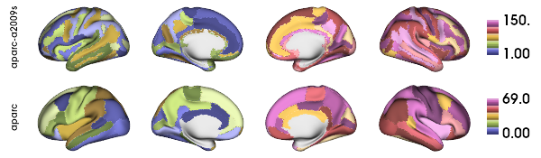
Anatomy based parcellations

Desikan-Killiany (aka Freesurfer aparc)

Desikan, R. S., Ségonne, F., Fischl, B., Quinn, B. T., Dickerson, B. C., Blacker, D., … & Albert, M. S. (2006). An automated labeling system for subdividing the human cerebral cortex on MRI scans into gyral based regions of interest. Neuroimage, 31(3), 968-980.

Dextrieux (aka Freesurfer aparc-a2009s)

Destrieux, C., Fischl, B., Dale, A., & Halgren, E. (2010). Automatic parcellation of human cortical gyri and sulci using standard anatomical nomenclature. Neuroimage, 53(1), 1-15.

# fsaverage5 | Plot parcellations
plot_hemispheres(fs5_lh, fs5_rh, array_name=surf_fs5[0:2], size=(600, 175), cmap='tab20b',
                 embed_nb=True, label_text={'left':parc[0:2]}, color_bar='right',
                 zoom=1.5, nan_color=nan_col)

# fsLR-32k | Plot parcellations
plot_hemispheres(f32k_lh, f32k_rh, array_name=surf_32k[0:2], size=(600, 175), cmap='tab20b',
                 embed_nb=True, label_text={'left':parc[0:2]}, color_bar='right',
                 zoom=1.5, nan_color=nan_col)

Histology based parcellation

Economo-Koskinas

Scholtens, L. H., de Reus, M. A., de Lange, S. C., Schmidt, R., & van den Heuvel, M. P. (2018). An mri von economo–koskinas atlas. NeuroImage, 170, 249-256.

# Plot parcellations fsaverage5
plot_hemispheres(fs5_lh, fs5_rh, array_name=surf_fs5[2], size=(600, 87), cmap='tab20',
                 embed_nb=True, label_text={'left':[parc[2]]}, color_bar='right',
                 zoom=1.5, nan_color=nan_col)

# Plot parcellations fsLR32k
plot_hemispheres(f32k_lh, f32k_rh, array_name=surf_32k[2], size=(600, 87), cmap='tab20',
                 embed_nb=True, label_text={'left':[parc[2]]}, color_bar='right',
                 zoom=1.5, nan_color=nan_col)

Multimodal based parcellation

Glasser

Glasser, M. F., Coalson, T. S., Robinson, E. C., Hacker, C. D., Harwell, J., Yacoub, E., … & Smith, S. M. (2016). A multi-modal parcellation of human cerebral cortex. Nature, 536(7615), 171-178.

# Plot parcellations
plot_hemispheres(fs5_lh, fs5_rh, array_name=surf_fs5[3], size=(600, 87), cmap='tab20c',
                 embed_nb=True, label_text={'left':[parc[3]]}, color_bar='right',
                 zoom=1.5, nan_color=nan_col)

# Plot parcellations
plot_hemispheres(f32k_lh, f32k_rh, array_name=surf_32k[3], size=(600, 87), cmap='tab20c',
                 embed_nb=True, label_text={'left':[parc[3]]}, color_bar='right',
                 zoom=1.5, nan_color=nan_col)

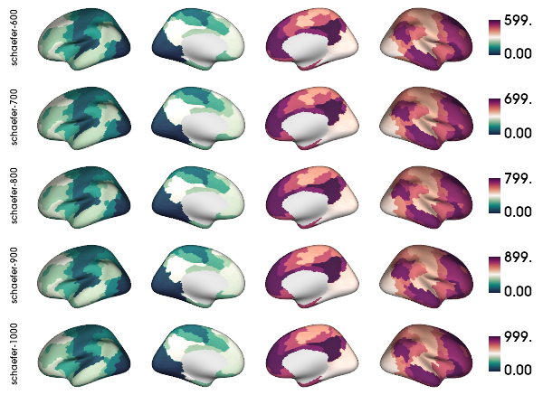
Functional based parcellation

Schaefer 100-1000

Schaefer, A., Kong, R., Gordon, E. M., Laumann, T. O., Zuo, X. N., Holmes, A. J., … & Yeo, B. T. (2018). Local-global parcellation of the human cerebral cortex from intrinsic functional connectivity MRI. Cerebral cortex, 28(9), 3095-3114.

# Plot parcellations
plot_hemispheres(fs5_lh, fs5_rh, array_name=surf_fs5[4:9], size=(600, 437), cmap='cmo.curl',
                 embed_nb=True, label_text={'left':parc[4:9]}, color_bar='right',
                 zoom=1.5, nan_color=nan_col)

# Plot parcellations
plot_hemispheres(f32k_lh, f32k_rh, array_name=surf_32k[4:9], size=(600, 437), cmap='cmo.curl',
                 embed_nb=True, label_text={'left':parc[4:9]}, color_bar='right',
                 zoom=1.5, nan_color=nan_col)

# Plot parcellations
plot_hemispheres(fs5_lh, fs5_rh, array_name=surf_fs5[9:14], size=(600, 437), cmap='cmo.curl',
                 embed_nb=True, label_text={'left':parc[9:14]}, color_bar='right',
                 zoom=1.5, nan_color=nan_col)

# Plot parcellations
plot_hemispheres(f32k_lh, f32k_rh, array_name=surf_32k[9:14], size=(600, 437), cmap='cmo.curl',
                 embed_nb=True, label_text={'left':parc[9:14]}, color_bar='right',
                 zoom=1.5, nan_color=nan_col)

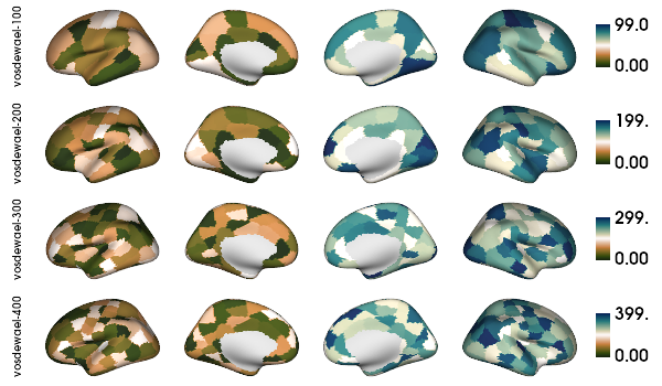
Pseudo-random parcellation based on `Desikan Killiany`

DK-random 100-500

vosdewael parcellations are semi-random subparcellations of Desikan Killiany, obtained by spliting in two the bigest parcel iterativelly until the desired number of parcels is reached.

# Plot parcellations
plot_hemispheres(fs5_lh, fs5_rh, array_name=surf_fs5[14:18], size=(600, 350), cmap='cmo.tarn',
                 embed_nb=True, label_text={'left':parc[14:18]}, color_bar='right',
                 zoom=1.5, nan_color=nan_col)

# Plot parcellations
plot_hemispheres(f32k_lh, f32k_rh, array_name=surf_32k[14:18], size=(600, 350), cmap='cmo.tarn',
                 embed_nb=True, label_text={'left':parc[14:18]}, color_bar='right',
                 zoom=1.5, nan_color=nan_col)

Parcellated Connectomes

Define functions to load each connectome

def load_mpc(File, Ndim):
    """Loads and process a MPC"""

    # load the matrix
    mtx_mpc = nib.load(File).darrays[0].data

    # Mirror the matrix
    MPC = np.triu(mtx_mpc,1)+mtx_mpc.T

    # Remove the medial wall
    MPC = np.delete(np.delete(MPC, 0, axis=0), 0, axis=1)
    MPC = np.delete(np.delete(MPC, Ndim, axis=0), Ndim, axis=1)

    return(MPC)

def load_fc(File, Ndim, parc=''):
    """Loads and process a functional connectome"""

    # load the matrix
    mtx_fs = nib.load(File).darrays[0].data

    # slice the matrix remove subcortical nodes and cerebellum
    FC = mtx_fs[49:, 49:]

    # Fisher transform
    FCz = np.arctanh(FC)

    # replace inf with 0
    FCz[~np.isfinite(FCz)] = 0

    # Mirror the matrix
    FCz = np.triu(FCz,1)+FCz.T
    return(FCz)

def load_gd(File, Ndim):
    """Loads and process a GD"""

    # load the matrix
    mtx_gd = nib.load(File).darrays[0].data

    # Remove the Mediall Wall
    mtx_gd = np.delete(np.delete(mtx_gd, 0, axis=0), 0, axis=1)
    GD = np.delete(np.delete(mtx_gd, Ndim, axis=0), Ndim, axis=1)

    return(GD)

def load_sc(File, Ndim, log_transform=True):
    """Loads and process a structura connectome"""

    # load the matrix
    mtx_sc = nib.load(File).darrays[0].data

    # Mirror the matrix
    if log_transform != True:
        mtx_sc = np.triu(mtx_sc,1)+mtx_sc.T
    else:
        mtx_sc = np.log(np.triu(mtx_sc,1)+mtx_sc.T)
    mtx_sc[np.isneginf(mtx_sc)] = 0

    # slice the matrix remove subcortical nodes and cerebellum
    SC = mtx_sc[49:, 49:]
    SC = np.delete(np.delete(SC, Ndim, axis=0), Ndim, axis=1)

    # replace 0 values with almost 0
    SC[SC==0] = np.finfo(float).eps

    return(SC)

Load connectomes function

Now, let’s create a function to load the connectomes and get the column mean of each modality including the FC.

def load_connectomes(connectome_type, parc, subjectDir, subjectID):
    """
    Load the specified connectome type and return roi_32k and roi_fs5.

    Parameters:
    connectome_type (str): Type of connectome to load. Options are 'GD', 'SC', 'MPC', 'FC'.
    subjectDir (str): Directory containing the subject data.
    subjectID (str): Subject ID.

    Returns:
    tuple: roi_32k and roi_fs5 arrays if successful, None otherwise.
    """

    # Empty list of surface plots
    roi_fs5 = [None] * len(parc)
    roi_32k = [None] * len(parc)

    for i, atlas in enumerate(parc):

        # Load fsaverage5 labels
        labels_fs5, mask_fs5, Ndim = load_annot(atlas, surf='fsaverage5')

        # Load fsLR-32k labels
        labels_32k, mask_32k, _ = load_annot(atlas, surf='fsLR-32k')

        try:
            if connectome_type == 'GD':
                # Load Geodesic Distance connectome
                file = f'{subjectDir}/dist/{subjectID}_atlas-{atlas}_GD.shape.gii'
                mtx = load_gd(file, Ndim)
            elif connectome_type == 'SC':
                # Load Structural Connectome
                file = f'{subjectDir}/dwi/connectomes/{subjectID}_space-dwi_atlas-{atlas}_desc-iFOD2-40M-SIFT2_full-connectome.shape.gii'
                mtx = load_sc(file, Ndim)
            elif connectome_type == 'MPC':
                # Load MPC
                acq_mpc = 'T1map'
                file = f'{subjectDir}/mpc/acq-{acq_mpc}/{subjectID}_atlas-{atlas}_desc-MPC.shape.gii'
                mtx = load_mpc(file, Ndim)
            elif connectome_type == 'FC':
                # Load Functional Connectome
                acq_func = 'desc-me_task-rest_bold'
                file = f'{subjectDir}/func/{acq_func}/surf/{subjectID}_atlas-{atlas}_desc-FC.shape.gii'
                mtx = load_fc(file, Ndim)
            else:
                raise ValueError("Invalid connectome type. Choose from 'GD', 'SC', 'MPC', 'FC'.")

            # Column sum
            mtx_s = np.sum(mtx, axis=0)

            # Map labels to surface fsaverage5
            roi_fs5[i] = map_to_labels(mtx_s, labels_fs5, fill=np.nan, mask=mask_fs5)

            # Map labels to surface fsLR-32k
            roi_32k[i] = map_to_labels(mtx_s, labels_32k, fill=np.nan, mask=mask_32k)

        except Exception as e:
            print(f"Error loading {connectome_type} connectome for atlas {atlas}: {e}")
            continue

    return roi_fs5, roi_32k

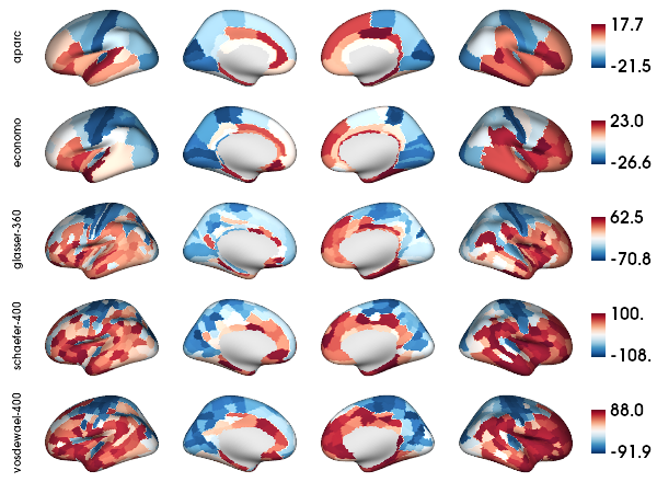
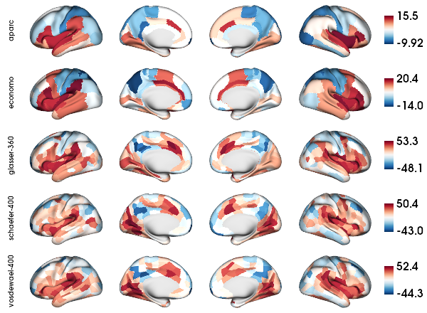
GD Connectomes `fsLR-32k`

# Parcellations to load
parc = ['aparc', 'economo', 'glasser-360', 'schaefer-400', 'vosdewael-400']
N = len(parc)

# Load the connectome row sum for each parcellation
roi_fs5, roi_32k = load_connectomes('GD', parc, subjectDir, subjectID)

# Plot parcellations
plot_hemispheres(f32k_lh, f32k_rh, array_name=roi_32k[0:N], size=(600, 88*N), cmap='RdBu_r',
                 embed_nb=True, label_text={'left':parc[0:N]}, color_bar='right',
                 zoom=1.5, nan_color=nan_col)

GD Connectomes `fsaverage5`

# Plot parcellations
plot_hemispheres(fs5_lh, fs5_rh, array_name=roi_fs5[0:N], size=(600, 88*N), cmap='RdBu_r',
                 embed_nb=True, label_text={'left':parc[0:N]}, color_bar='right',
                 zoom=1.5, nan_color=nan_col)

Structural Connectomes `fsLR-32k`

# Load the connectome row sum for each parcellation
roi_fs5, roi_32k = load_connectomes('SC', parc, subjectDir, subjectID)

# Plot parcellations
plot_hemispheres(f32k_lh, f32k_rh, array_name=roi_32k[0:N], size=(600, 88*N), cmap='RdBu_r',
                 embed_nb=True, label_text={'left':parc[0:N]}, color_bar='right',
                 zoom=1.5, nan_color=nan_col)

Structural Connectomes `fsaverage5`

# Plot parcellations
plot_hemispheres(fs5_lh, fs5_rh, array_name=roi_fs5[0:N], size=(600, 88*N), cmap='RdBu_r',
                 embed_nb=True, label_text={'left':parc[0:N]}, color_bar='right',
                 zoom=1.5, nan_color=nan_col)

MPC Connectomes `fsLR-32k`

# Load the connectome row sum for each parcellation
roi_fs5, roi_32k = load_connectomes('MPC', parc, subjectDir, subjectID)

# Plot parcellations
plot_hemispheres(f32k_lh, f32k_rh, array_name=roi_32k[0:N], size=(600, 88*N), cmap='RdBu_r',
                 embed_nb=True, label_text={'left':parc[0:N]}, color_bar='right',
                 zoom=1.5, nan_color=nan_col)

MPC Connectomes `fsaverage5`

# Plot parcellations

plot_hemispheres(fs5_lh, fs5_rh, array_name=roi_fs5[0:N], size=(600, 88*N), cmap='RdBu_r',
                 embed_nb=True, label_text={'left':parc[0:N]}, color_bar='right',
                 zoom=1.5, nan_color=nan_col)

FC Connectomes `fsLR-32k`

# Load the connectome row sum for each parcellation
roi_fs5, roi_32k = load_connectomes('FC', parc, subjectDir, subjectID)

# Plot parcellations
plot_hemispheres(f32k_lh, f32k_rh, array_name=roi_32k[0:N], size=(600, 88*N), cmap='RdBu_r',
                 embed_nb=True, label_text={'left':parc[0:N]}, color_bar='right',
                 zoom=1.5, nan_color=nan_col)

FC Connectomes `fsaverage5`

# Plot parcellations

plot_hemispheres(fs5_lh, fs5_rh, array_name=roi_fs5[0:N], size=(600, 88*N), cmap='RdBu_r',
                 embed_nb=True, label_text={'left':parc[0:N]}, color_bar='right',
                 zoom=1.5, nan_color=nan_col)